Chapter 13Smoothing by optimization
When a function is non-differentiable (or worse, discontinuous), a reasonable approach is to replace it by a differentiable approximation (or at least, by a continuous relaxation). We refer to the process of transforming a non-differentiable function into a differentiable one as “smoothing” the original function. In this chapter, we begin by reviewing a smoothing technique based on infimal convolution. We then review an equivalent dual approach, based on the Legendre-Fenchel transform. We illustrate how to apply these techniques to compute smoothed ReLUs and smoothed max operators, as well as continuous relaxations of step functions and argmax operators.
13.1 Primal approach
We first review how to smooth functions in the original, primal space of the function, using the infimal convolution and more particularly the Moreau envelope, a.k.a. Moreau-Yoshida regularization. In this chapter, we consider functions taking potentially infinite positive values, that is, functions taking values in the half-extended real line . For a function , we define its domain as
13.1.1 Infimal convolution
Sometimes abbreviated inf-conv, the infimal convolution between two functions and creates a new function . It is defined as follows.
Definition 13.1 (Infimal convolution)
The infimal convolution between two functions and is defined by
It is easy to check that the three definitions are indeed equivalent, by using the change of variable , which is a location-scale transform; see Section 12.4.1.
The infimal convolution can be seen as a counterpart of the usual convolution, in which integration has been replaced by minimization (hence its name). Similarly to the classical convolution, it is commutative, meaning that for all , we have
Computing the infimal convolution involves the resolution of a minimization problem, that may or may not enjoy an analytical solution. Some examples are given in Table 13.1.
Existence
The infimal convolution exists if the infimum is finite (Bauschke and Combettes, 2017, Proposition 12.6). A sufficient condition to achieve this is that is convex for all . However, this is not a necessary condition. For example, the infimum can be finite even if or are nonconvex, for example if their domain is a compact set.
Infimal convolution with a regularization function
When a function is non-differentiable, a commonly-used technique is to replace it by its infimal convolution , with some regularization . The most used regularization is the squared -norm, leading to the Moreau envelope, as we now review.
Table 13.1: Examples of infimal convolutions. We use to denote the indicator function of the set .
13.1.2 Moreau envelope
When , the infimal convolution gives the so-called Moreau envelope of , which is also known as Moreau-Yoshida regularization of .
Definition 13.2 (Moreau envelope)
Given a function , its Moreau envelope is defined as
Intuitively, the Moreau envelope is the minimal value over of a trade-off between staying close to the input according to the proximity term and minimizing . Provided that the minimizer exists and is unique, we can define the associated proximal operator of as In other words, we have for well defined,
Properties
A crucial property of the Moreau envelope is that for any convex function , it is always a smooth function, even when itself is not smooth. By smooth, we formally mean that the resulting function is differentiable everywhere with Lipschitz-continuous gradients. We say -smooth, if the gradients are -Lipschitz continuous. Such a property can determine the efficiency of optimization algorithms as reviewed in Section 15.4. We recap below useful properties of the Moreau envelope.
Proposition 13.1 (Properties of Moreau envelope)
Let .
Smoothness: If is convex, the function is -smooth.
Gradient: Provided that is well-defined on , the gradient of the Moreau envelope can be expressed in terms of the proximal operator as
Moreau decomposition: If is convex, then for any , we have the following identity where is the convex conjugate of , detailed in Section 13.2. In particular, we get
Convexity: is convex if is convex.
Infimums coincide: has the same infimum as the original function :
Proof
This is best seen using the dual approach detailed in Section 13.3.
This follows from Danskin’s theorem, reviewed in Section 11.2.
See, e.g., Bauschke and Combettes (2017, Theorem 14.3).
This follows from the fact that the infimum of a jointly convex function is convex.
We have
◻
Examples
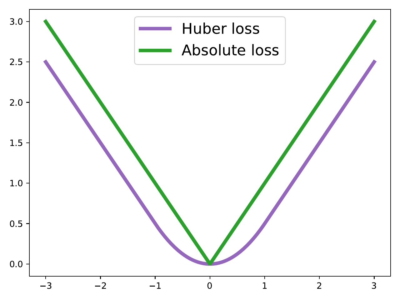
Figure 13.1: The Huber loss is the Moreau envelope of the absolute loss.
To illustrate smoothing from the Moreau envelope perspective, we show how to smooth the -norm. In this case, we obtain an analytical expression for the Moreau envelope.
Example 13.1 (Smoothing the -norm via infimal convolution)
We wish to smooth . The corresponding proximal operator is the soft-thresholding operator (see Section 16.4), Using Eq. (13.1) and after some algebraic manipulations, we obtain where we defined the Huber loss This is illustrated in Fig. 13.1 with .
We also illustrate in Fig. 13.2 that the Moreau envelope of nonconvex functions can be approximately computed numerically.
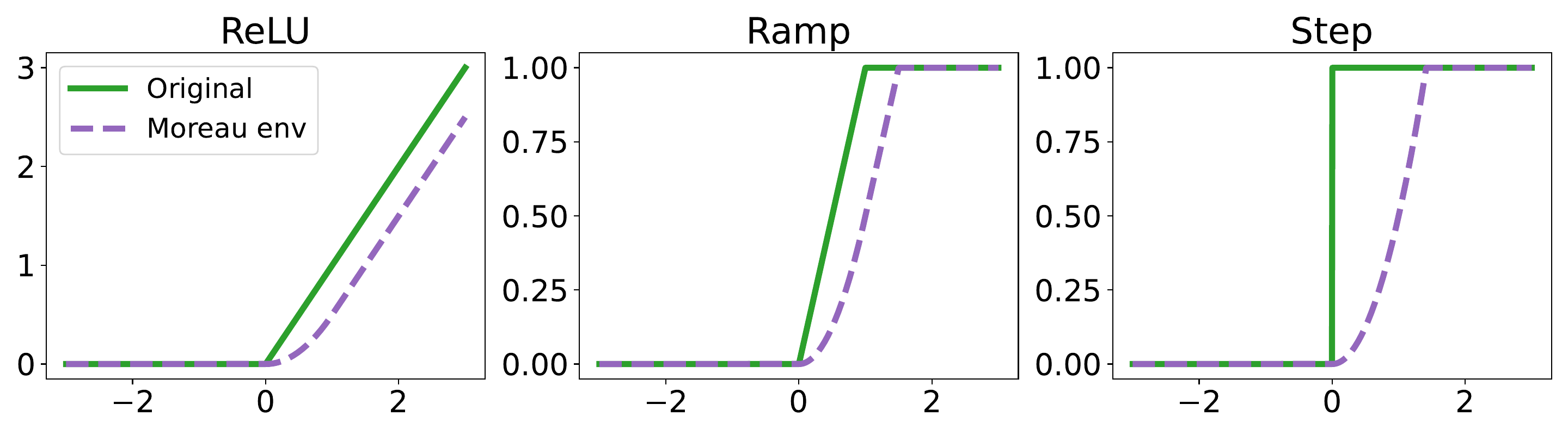
Figure 13.2: The Moreau envelope is not limited to convex functions. For instance, the ramp function is continuous but nonconvex, and the step function is not only nonconvex but also discontinuous. In this figure, we approximately computed the infimum over in Definition 13.2 by restricting the search on a finite grid, in a closed interval.
13.1.3 Vector-valued functions
The Moreau envelope is defined by . As such, it is limited to scalar-valued functions . To extend the Moreau envelope to vector-valued functions , where and for , we may choose to smooth each separately to define where This approach requires solving separate minimization problems and performs the smoothing of each output coordinate independently. From Proposition 2.9, we then have that the VJP of with any direction is In the particular case , we obtain
An alternative was proposed by Roulet and Harchaoui (2022). For a differentiable function , we recall that the VJP of with a direction reads where we defined the scalar-valued function . As a result, if is non-differentiable, a natural idea is to approximate its VJP (had it existed) by the gradient of the Moreau envelope This requires solving a single optimization problem, independently of the number of outputs . Moreover, for , this recovers as a special case.
This approach allows in principle to perform reverse-mode autodiff (gradient backpropagation) on a neural network whose layers use the Moreau envelope. Indeed, following Proposition 13.1, the approximate VJP of with a direction is given by where is the solution of the minimization problem in Eq. (13.2). However, we emphasize that this minimization problem could be difficult to solve in general. Indeed, when performing gradient backpropagation, the direction is not necessarily non-negative, therefore the function being minimized in Eq. (13.2) could be nonconvex, even if each is convex. Another potential caveat is that the direction influences the smoothing strength, while in principle we should be able to smooth a function independently of whether we compute its VJP or not. To see that, for example in the particular case , one easily checks that for , we get Smoothing vector-valued functions by Moreau envelope (or more generally, by infimal convolution) remains an open area of research. We will see in Chapter 14 that smoothing by convolution more naturally supports vector-valued functions.
13.2 Legendre–Fenchel transforms, convex conjugates
The Legendre-Fenchel transform, a.k.a. convex conjugate, is a way to turn a function into a new function, denoted . We now review it in detail, as it plays a major role for the dual approach to smoothing.
13.2.1 Definition
Consider the class of affine functions of the form These functions are parametrized by their slope and their intercept . Now, suppose we fix . Given a function , affine lower bounds of are all the functions of such that satisfies for all , The tightest lower bound is then defined by such that where we recall that the domain of is defined by This leads to the definition of Legendre-Fenchel transform, a.k.a. convex conjugate.
Definition 13.3 (Legendre-Fenchel transform, convex conjugate)
Given a function , its convex conjugate is defined by
We use a rather than a to indicate that is potentially . Following the previous discussion, is the intercept of the tightest affine lower bound with slope of . This is illustrated in Fig. 13.3.
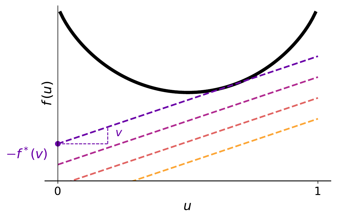
Figure 13.3: For a fixed slope , the function is the tightest affine lower bound of with slope .
The Legendre-Fenchel transform is a function transformation, as it produces a new function . It can be seen as a dual representation of a function: instead of representing a convex function by its graph for , we can represent it by the set of tangents with slope and intercept for , as illustrated in Fig. 13.4. As the name “convex conjugate” indicates, it is convex, even if the original function is not.
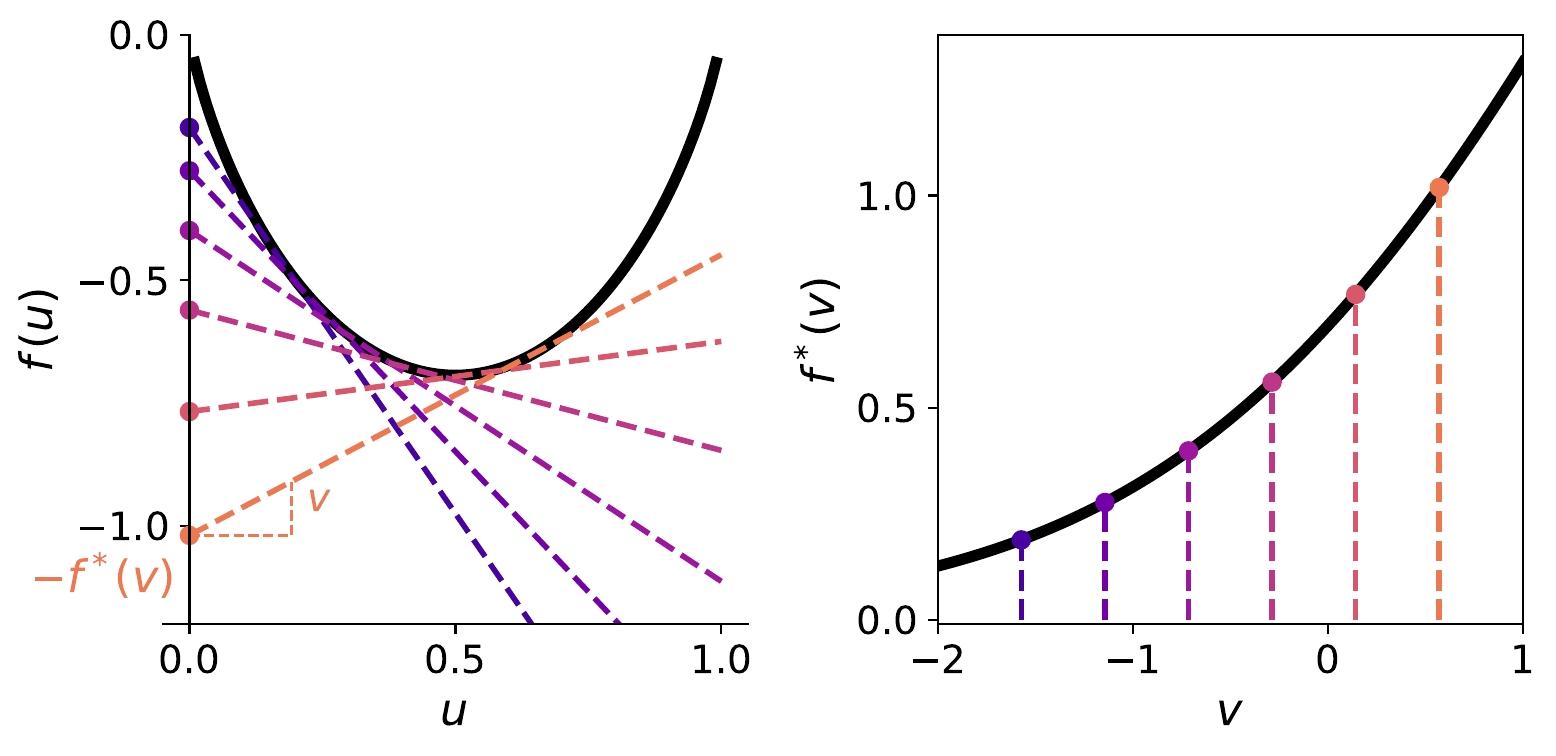
Figure 13.4: Left: instead of representing a convex function by its graph for , we can represent it by the set of tangents with slope and intercept for . Right: by varying the slope of all possible tangents, we obtain a function of the slope rather than of the original input . The colors of the tangents on the left are chosen to match the colors of the vertical lines on the right.
13.2.2 Closed-form examples
Computing involves the resolution of a maximization problem, which could be difficult in general without assumption on . In some cases, however, we can compute an analytical expression, as we now illustrate.
Example 13.2 (Analytical conjugate examples)
When , with , the conjugate is Setting the gradient to zero, we obtain . Plugging back, we therefore obtain Therefore, in this case.
When , with , the minimizer of is and the conjugate is
See for instance Boyd and Vandenberghe (2004) or Beck (2017) for many more examples.
Constraining the domain
We can incorporate constraints using an indicator function with values in the extended real line ,
Example 13.3 (Incorporating constraints)
If , where is a convex set, then which is known as the support function of . The corresponding argmax (assuming that it exists), is known as the linear maximization oracle (LMO) of . As another example, if then We postpone a proof to Proposition 13.9.
13.2.3 Properties
The conjugate enjoys several useful properties, that we now summarize.
Proposition 13.2 (Convex conjugate properties)
Convexity: is a convex function for all (even if is nonconvex).
Fenchel-Young inequality: for all
Gradient: if the supremum in Definition 13.3 is uniquely achieved, then is differentiable at and its gradient is Otherwise, is sub-differentiable at and we get a sub-gradient instead.
Maps: If and are differentiable, then
Biconjugate: if and only if is convex and closed (i.e., its sublevel sets form a closed set), otherwise .
Proof
This follows from the fact that is convex if is convex in . Note that this is true even if is nonconvex in . Here, , which is affine in and therefore convex in .
This follows immediately from Definition 13.3.
This follows from Danskin’s theorem, reviewed in Section 11.2. Another way to see this is by observing that where . Subtracting the two, we obtain Now, using that is convex and Definition 15.6, we obtain that .
See, e.g., Bauschke and Combettes (2017, Proposition 16.10).
See Boyd and Vandenberghe (2004, Section 3.3).
◻
13.2.4 Conjugate calculus
While deriving a convex conjugate expression can be difficult in general, in some cases, it is possible to use simple rules to derive conjugates in terms of other conjugates.
Proposition 13.3 (Conjugate calculus rules)
Separable sum of functions: if , then
Scalar multiplication: if , for , then
Addition to an affine function and translation: if , then
Composition with an invertible linear map: if , where is an invertible linear map, then
Non-separable sum of functions: if and are convex functions, then , where is the infimal convolution operator.
13.2.5 Fast Legendre transform
When an analytical expression is not available, we can resort to numerical schemes to approximately compute the transform / conjugate. When is convex, because is concave, the maximization in Definition 13.3 is that of a concave function. Therefore, the conjugate can be computed to arbitrary precision in polynomial time using classical iterative algorithms for constrained optimization such as projected gradient descent (Section 16.3) or conditional gradient a.k.a. Frank-Wolfe (Jaggi, 2013). Without convexity assumption on , can be approximated by where is a discrete grid of values. We can then compute for several inputs using the linear-time Legendre transform algorithm (Lucet, 1997), where is another discrete grid. The complexity is , which is linear in the grid sizes. However, the grid sizes are typically , for equally-distributed points in each of the dimensions. Therefore, this approach is limited to small-dimensional settings, e.g., .
13.3 Dual approach
Previously, we presented how to smooth a function by performing its infimal convolution with a primal-space regularization . We now present how to smooth a function by regularizing its Legendre-Fenchel transform (convex conjugate) instead. This dual, equivalent approach, is often mathematically more convenient.
13.3.1 Duality between strong convexity and smoothness
We begin by stating a well-known result that will underpin this whole section: smoothness and strong convexity are dual to each other (Beck, 2017; Hiriart-Urruty and Lemaréchal, 1993; Kakade et al., 2009; Zhou, 2018).
Proposition 13.4 (Duality between strong convexity and smoothness)
is -strongly convex w.r.t. the norm over if and only if is -smooth w.r.t. the dual norm over .
For a review of the notions of smoothness and strong convexity, see Section 15.4. We give two examples of strongly-convex and smooth conjugate pairs in Table 13.2.
Table 13.2: Examples of strongly-convex and smooth conjugate pairs.
| Function | Norm | Domain | Conjugate | Dual norm | Dual domain |
|---|---|---|---|---|---|
13.3.2 Smoothing by dual regularization
The duality between smoothness and strong convexity suggests a generic approach in order to smooth a function , by going through the dual space.
Compute the conjugate :
Add strongly-convex regularization to the conjugate:
Go back to the primal space, by computing the conjugate of :
Note that and belong to different spaces, i.e., and . Following Proposition 13.4, if is -strongly convex, then is -smooth. Furthermore, following Proposition 13.2, is convex, even if is nonconvex. Therefore, is a smooth and convex relaxation of .
Steps and are the most challenging, as they both require the derivation of a conjugate. While an analytical solution may not exist in general, in some simple cases, there is, as we now illustrate.
Example 13.4 (Smoothing the -norm via dual regularization)
We revisit Example 13.1, this time from the dual perspective. We wish to smooth out the -norm .
Compute the conjugate. The conjugate of any norm is the indicator function of the dual norm’s unit ball (see e.g. Boyd and Vandenberghe (2004, Example 3.26)). The dual norm of is . Moreover, Recalling that is the indicator function of , we obtain
Adding strongly-convex regularization. We add quadratic regularization to define
Going back to the primal. where .
We therefore indeed recover the Huber loss from Example 13.1.
ReLU functions can be smoothed out in a similar way, as we see in more details in Section 13.4.
The dual approach allows us to easily bound the smoothed function in terms of the original function.
Proposition 13.5 (Bounding the smoothed function)
Let be a closed convex function. Let be a convex function. If is such that for all , then for all ,
Proof
Let us define where we recall that . We then have for all Similarly, Combining the two with for all , we obtain ◻
Remark 13.1 (The gradient is differentiable almost everywhere)
From Proposition 13.2, the gradient of equals If is strongly convex, then is smooth, meaning that is Lipschitz continuous. From Rademacher’s theorem reviewed in Section 2.7.1, is then differentiable almost everywhere (that is, is twice differentiable almost everywhere). We use this property in the sequel to define continuous differentiable almost everywhere relaxations of step functions and argmax operators.
13.3.3 Equivalence between primal and dual regularizations
So far, we saw two approaches to obtain a smooth approximation of a function . The first approach is based on the infimal convolution , where denotes primal regularization. The second approach is based on regularizing the Legendre-Fenchel transform (convex conjugate) of with some dual regularization , to define . It turns out that both approaches are equivalent.
Proposition 13.6 (Equivalence between primal and dual regularizations)
Let and , both convex and closed. Then, with .
Proof
We have If and are convex, we have (Beck, 2017, Theorem 4.17). Using and gives the desired result using that and since both are convex and closed (see Proposition 13.2). ◻
In particular, with , this shows that the Moreau envelope can equivalently be written as Given the equivalence between the primal and dual approaches, using one approach or the other is mainly a matter of mathematical or algorithmic convenience, depending on the case.
In this book, we focus on applications of smoothing techniques to differentiable programming. For applications to non-smooth optimization, see (Beck and Teboulle, 2012; Nesterov; 2005).
13.3.4 Regularization scaling
Dual approach
If is -strongly convex, then is a -smooth approximation of the original function . To control the smoothness of the approximation, we regularize with for , defining Consequently, the gradient is given by This formulation works for any closed convex . The approximation error induced by the smoothing can be quantified using Proposition 13.5. Provided that for all , we have
Remark 13.2 (Homogeneous case)
In the special case where is positively homogeneous of degree (e.g., a norm), its conjugate is an indicator function satisfying . In this specific setting, we recover the scaling relationships:
Primal approach
Following Definition 13.2, if we use dual regularization , where controls the regularization strength, assuming is convex, the corresponding primal regularization is and we have In the particular case , we have We therefore get
13.3.5 Generalized entropies
A natural choice of dual regularization , when is a discrete probability distribution, is a negative entropy function, also known as negentropy. Since negentropies play a major role in smoothed max operators, we discuss them in detail here.
Information content and entropy
An entropy function measures the amount of “surprise” of a random variable or equivalently of a distribution. To define an entropy, we must first define the information content of an event . The value returned by such a function should be if the probability of the event is , as there is no surprise. Conversely, information content should attain its maximal value if the probability of the event is , as it is maximally surprising. Furthermore, the more probable an event is, the less surprising it is. Therefore, when increases, should decrease. Overloading the notation, we also write the information content of the outcome of a random variable as the information content of the event ,
Given an information content function, we can then define the entropy of a random variable as the expected information content, Different definitions of information content lead to different definitions of entropy.
Shannon’s entropy
A definition of information content satisfying the criteria above is Indeed, , and is a decreasing function over . Using this information content definition leads to Shannon’s entropy (Shannon, 1948) We can therefore define the Shannon entropy of a discrete probability distribution as and use the corresponding negentropy as regularization The function is strongly convex w.r.t. over . However, it is not strongly convex over , since this is not a bounded set; see for instance (Blondel, 2019, Proposition 2). Since is added to in Eq. (13.3), we can therefore use this choice of to smooth out a function if .
Gini’s entropy
As an alternative, we can define information content as The factor is for later mathematical convenience. This again satisfies the criteria of an information content function. Indeed, i) when , ii) when , attains its maximum of iii) the function is decreasing w.r.t. . Using this information content definition leads to Gini’s entropy a.k.a. Gini index (Gini, 1912) We can use Gini’s negative entropy to define for all The function is strongly convex w.r.t. over . We can therefore use this choice of to smooth out a function if . This means that the set of functions that we can smooth out with Gini entropy is larger than the set of functions we can smooth out with Shannon entropy.
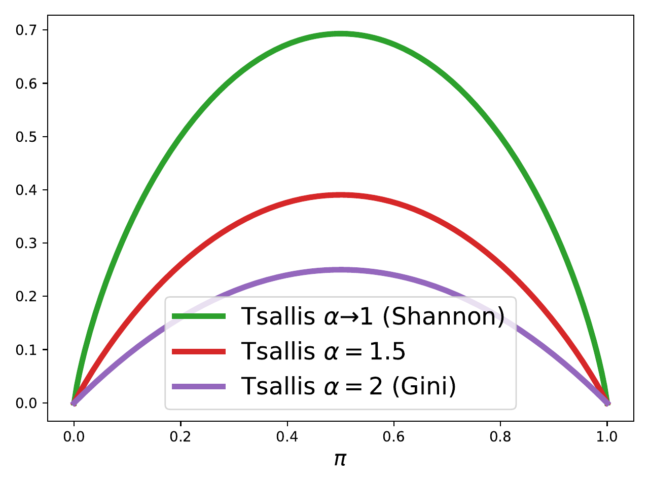
Figure 13.5: Tsallis entropies of the distribution , for . An entropy is a non-negative concave function that attains its maximum at the uniform distribution, here . A negative entropy, a.k.a. negentropy, can be used as a dual regularization function to smooth out a function when .
Tsallis entropies
Given , a more general information content definition is Using this definition leads to the Tsallis entropy (Tsallis, 1988) The Tsallis entropy recovers the Shannon entropy in the limit and the Gini entropy when . We can use the Tsallis negative entropy to define for all where is the -norm for () so that Tsallis entropies for (Shannon entropy), and (Gini entropy) are illustrated in Fig. 13.5 and Fig. 13.6.
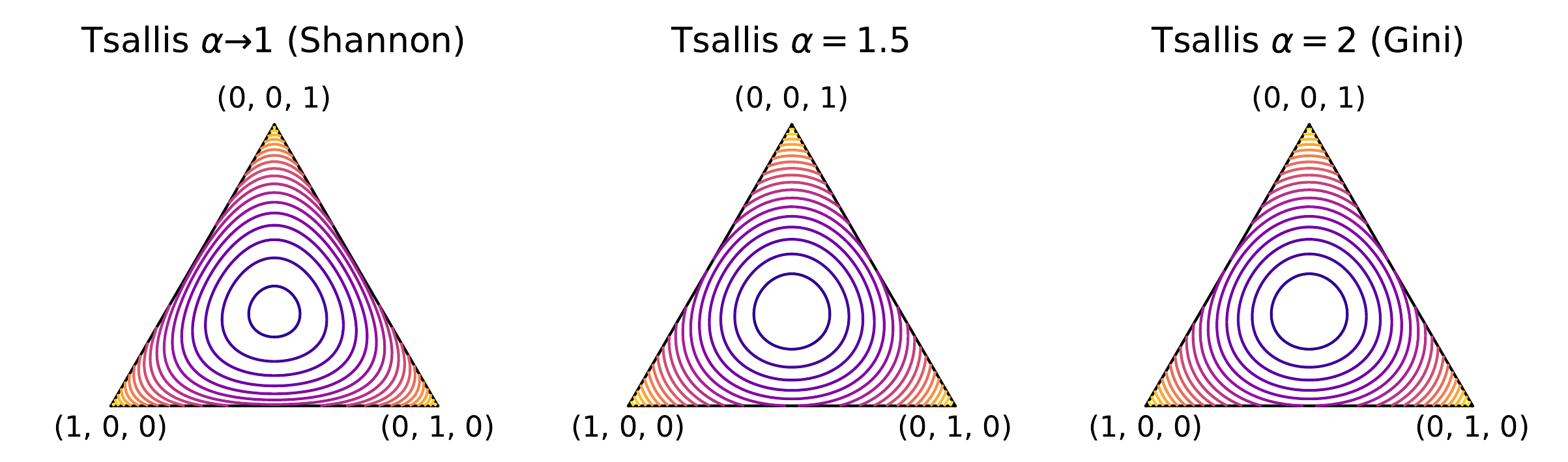
Figure 13.6: Contours of Tsallis entropies on the probability simplex.
Definition and properties of generalized entropies
So far, we saw how to define an entropy as the expected information content. However, generalized entropies (DeGroot, 1962; Grünwald and Dawid, 2004) do not necessarily need to take this form. We follow the definition of Blondel et al. (2020).
Definition 13.4 (Entropy function)
A function is an entropy if
if ,
is strictly concave,
for any permutation matrix .
This definition implies that is non-negative and is uniquely maximized by the uniform distribution (Blondel et al., 2020, Proposition 4). This is indeed what we expect from an entropy function. An example is the squared -norm entropy (Blondel et al., 2020) Since the squared -norm is strongly convex for (Ball et al., 2002), this entropy is strongly concave for and can therefore be used to smooth out functions.
We now illustrate how to apply these techniques to compute smoothed ReLUs and smoothed max operators, as well as continuous relaxations of step functions and argmax operators.
13.4 Smoothed ReLU functions
To demonstrate the application of the smoothing techniques discussed in this chapter, we begin by explaining how to smooth the ReLU function. The ReLU function is defined by We recall that in order to smooth a function by the dual approach, we calculate its conjugate , add regularization to it to obtain and then obtain by computing .
Here, we wish to smooth out . Its convex conjugate is To notice why, we observe that Indeed, since the objective is linear in , the maximum is attained at one of the extreme points of , so that we can replace the constraint with . This shows that the ReLU is exactly the support function of . Since the conjugate of the support function is the indicator function, we indeed obtain . We therefore have and for some choice of , we need to be able to compute
The softplus
If we use the regularizer , which comes from using Shannon’s negentropy with , we obtain This result is a special case of Proposition 13.9.
The sparseplus
If we use the regularizer , which comes from using Gini’s negentropy with with , we obtain See Fig. 13.8 (left figure) for a comparison of softplus and sparseplus.
13.5 Smoothed max operators
As a more elaborate application of the smoothing techniques discussed in this chapter, we explain how to smooth max operators. Smoothed max operators include smoothed ReLU functions as a special case.
13.5.1 Definition and properties
With a slight notation overloading, given a vector , we define its maximum as To obtain a smooth approximation of , we again apply the dual approach. The conjugate of is To notice why, we observe that the vertices of the probability simplex are the standard basis vectors . Since the objective is linear, we then have In other words, the maximum operator is exactly the support function of . Since the conjugate of the support function is the indicator function, we indeed obtain . We can therefore write and The smoothed max operator can be useful in a neural network, for example as a smoothed max pooling layer. Its properties have been studied in (Mensch and Blondel, 2018, Lemma 1), as we recall here for convenience.
Proposition 13.7 (Properties of )
The following properties hold.
Bounds: if for all , then for all .
Monotonicity: if (element-wise), then .
Commutativity: if for any permutation matrix and any , then for any permutation matrix .
Distributivity of : for all and all .
These properties are leveraged in (Mensch and Blondel, 2018) to create differentiable dynamic programs. We consider in the following two possible choices of leading to the softmax and sparsemax operators illustrated in Fig. 13.7.
Smoothed min operators
The minimum operator can be expressed in terms of the maximum operator, since for all , Given a smoothed max operator , we can therefore easily define a smoothed min operator as
13.5.2 Reduction to root finding
Computing for a general strongly-convex regularization involves the resolution of a maximum over probability simplex constraints. For convenience, let us define the notation The following proposition shows that we can reduce computing to solving a root equation involving .
Proposition 13.8 (Computing as root finding)
Suppose is strongly convex. For all , and where is the solution w.r.t. of the above , which satisfies the root equation
Proof
The idea is to keep the non-negativity constraint explicit, but to use a Lagrange multiplier for the equality constraint of the probability simplex. We then have where we used that we can swap the and the , since is convex-concave and is an affine constraint. The gradient follows from Danskin’s theorem. The root equation follows from computing the derivative of and setting it to zero. ◻
13.5.3 The softmax
When is Shannon’s negentropy, we obtain that is the softmax, already briefly discussed in Section 4.4.2.
Proposition 13.9 (Analytical expression of the softmax)
When , we get
Proof
Since , we have (i.e., the non-negativity constraint is redundant). From Example 13.2, we therefore have . From Proposition 13.8, where satisfies Since , we need to solve . We therefore get and therefore . ◻
Since for all , following Proposition 13.7, we get for all A unique property of the softmax, which is not the case of all operators, is that it supports associativity.
Proposition 13.10 (Associativity of the softmax)
For all ,
13.5.4 The sparsemax
Alternatively, choosing to be Gini’s negentropy leads to the sparsemax (Martins and Astudillo, 2016; Mensch and Blondel, 2018).
Proposition 13.11 (Variational formulation of sparsemax)
When , we have where
Proof
This follows from the fact that is up to a constant equal to and completing the square. ◻
Therefore, computing the sparsemax can use the sparseargmax (the Euclidean projection onto the probability simplex) as a building block. We discuss how to compute it in more detail in Section 13.7. Applying Proposition 13.8 gives an alternative formulation.
Proposition 13.12 (Sparsemax as root finding)
When , we have and satisfies
Proof
First, we compute the expression of . Setting the gradient of to zero and clipping, we obtain . Plugging back, we obtain . Using Proposition 13.8 proves the proposition’s first part. Setting the derivative w.r.t. to zero gives the second part. ◻
It can be shown (Condat, 2016; Duchi et al., 2008) that the exact solution is obtained by where is the largest such that and where we used the notation . As an alternative, we can also compute approximately using a bisection or by gradient descent w.r.t. .
For , since , we have Following Proposition 13.7, we therefore get for all
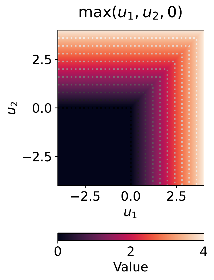
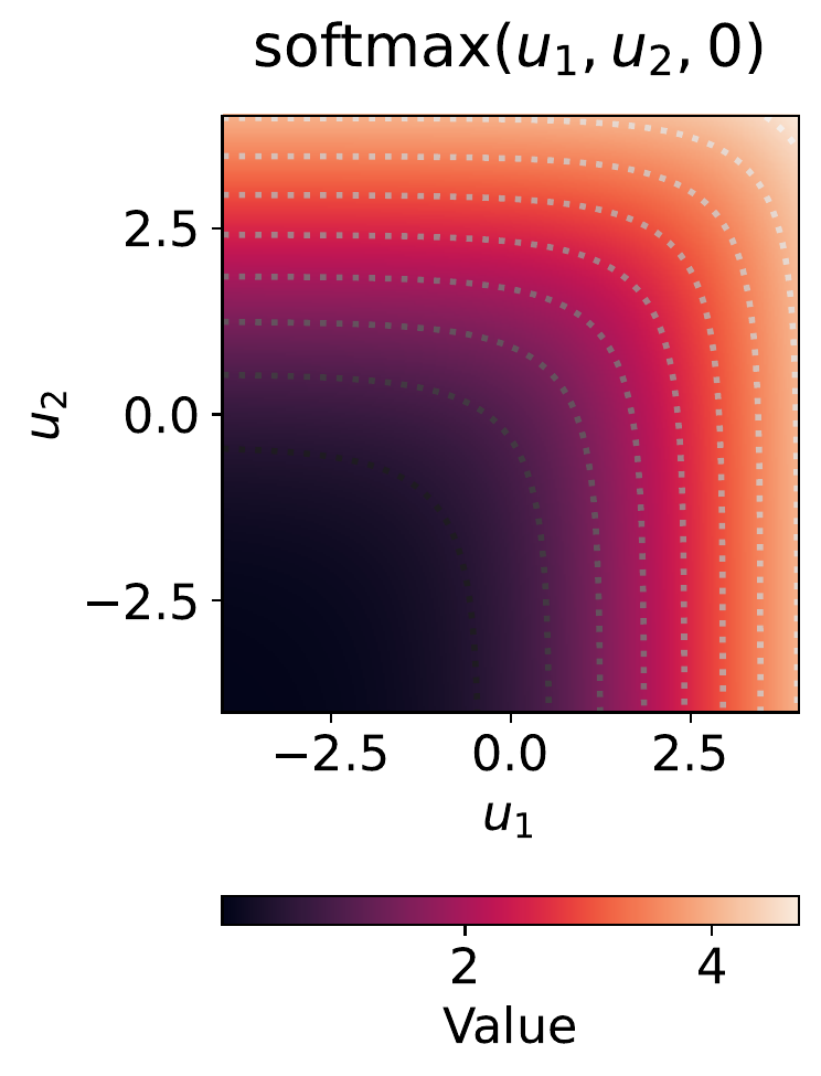
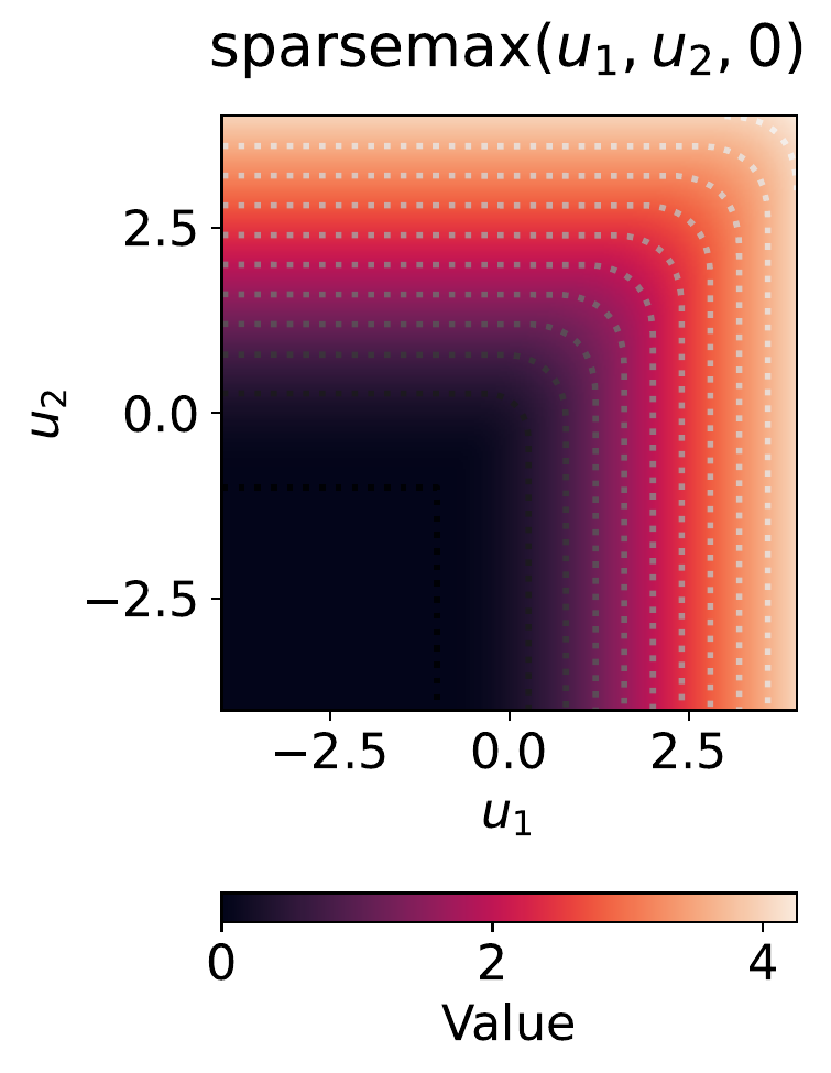
Figure 13.7: Max, softmax and sparsemax functions. The max function has non-smooth contour lines (set of points for some constant represented by dashed gray lines). The gradient along these contour lines switches suddenly at the corners of the contour lines switch. This shows that the max function is not differentiable everywhere, namely, non-differentiable on the set of points . The contour lines of the softmax and sparsemax functions on the other hand are smooth illustrating that these functions are smooth counterparts of the max function.
13.5.5 Recovering smoothed ReLU functions
Using the vector as input, the smoothed max operator recovers the smoothed ReLU: where we defined . With being Shannon’s negentropy, we recover ; with being Gini’s negentropy, we recover , that we used to smooth the ReLU.
13.6 Relaxed step functions (sigmoids)
We now turn to creating continuous relaxations of step functions. The binary step function, a.k.a. Heaviside step function, is defined by From Eq. (13.4), its variational form is We can therefore define the relaxation Notice that, unlike the case of the smoothed ReLU, it is a regularized argmax, not a regularized max. Following Remark 13.1, strongly convex regularization ensures that is a Lipschitz continuous function of and is therefore, at least, differentiable almost everywhere, unlike .
The logistic function
If we use the regularizer , we obtain the closed form This function is differentiable everywhere.
The sparse sigmoid
As an alternative, if we use , we obtain a piecewise linear sigmoid, Unlike the logistic function, it can reach the exact values or . However, the function has two kinks, where the function is non-differentiable.
Link between smoothed ReLU functions and sigmoids
It turns out that the three sigmoids we presented above (step, logistic, sparsesigmoid) are all equal to the derivative of their corresponding smoothed ReLU function: and more generally This is a consequence of Danskin’s theorem; see Example 11.2. We illustrate the smoothed ReLU functions and relaxed step functions (sigmoids) in Fig. 13.8.
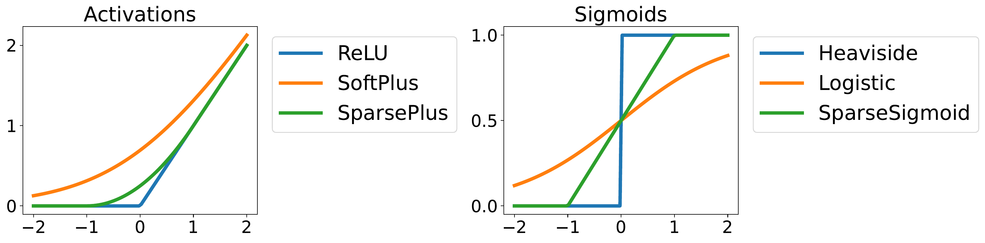
Figure 13.8: Smoothed ReLU functions and relaxed step functions (sigmoids). Differentiating the left functions gives the right functions.
13.7 Relaxed argmax operators
We now turn to argmax operators, which are a generalization of step functions. With a slight notation overloading, let us now define where is used to embed any integer into . Following the previous discussion, we have the variational form where the second equality uses that a linear function is maximized at one of the vertices of the simplex. This variational form suggests to define the relaxation Again, following Remark 13.1, is guaranteed to be, at least, a differentiable almost everywhere function of if is strongly convex.
Similarly to sigmoids, it turns out that these mappings are equal to the gradient of their corresponding smoothed max operator: This is again a consequence of Danskin’s theorem.
The softargmax
When using Shannon’s negative entropy , we obtain which is differentiable everywhere.
Proof
We know that and that . Differentiating gives . ◻
The sparseargmax
When using Gini’s entropy , which is up to a constant equal to , we obtain the sparseargmax (Martins and Astudillo, 2016) which is nothing but the Euclidean projection onto the probability simplex (see also Section 16.3). The Euclidean projection onto the probability simplex can be computed exactly using a median-finding-like algorithm. The complexity is expected time and worst-case time (Brucker, 1984; Condat, 2016; Duchi et al., 2008; Michelot, 1986). Computing the Euclidean projection onto the probability simplex boils down to computing given in Eq. (13.5). Once we computed it, we have As its name indicates, and as the above equation shows, sparseargmax is sparse, but it is only differentiable almost everywhere. Note that the operator is originally known as sparsemax (Martins and Astudillo, 2016), but this is a misnomer, as it is really an approximation of the argmax. Therefore, in analogy with the softargmax, we use the name sparseargmax. We compare the argmax, softmax and sparseargmax in Fig. 13.9 and Fig. 13.10.
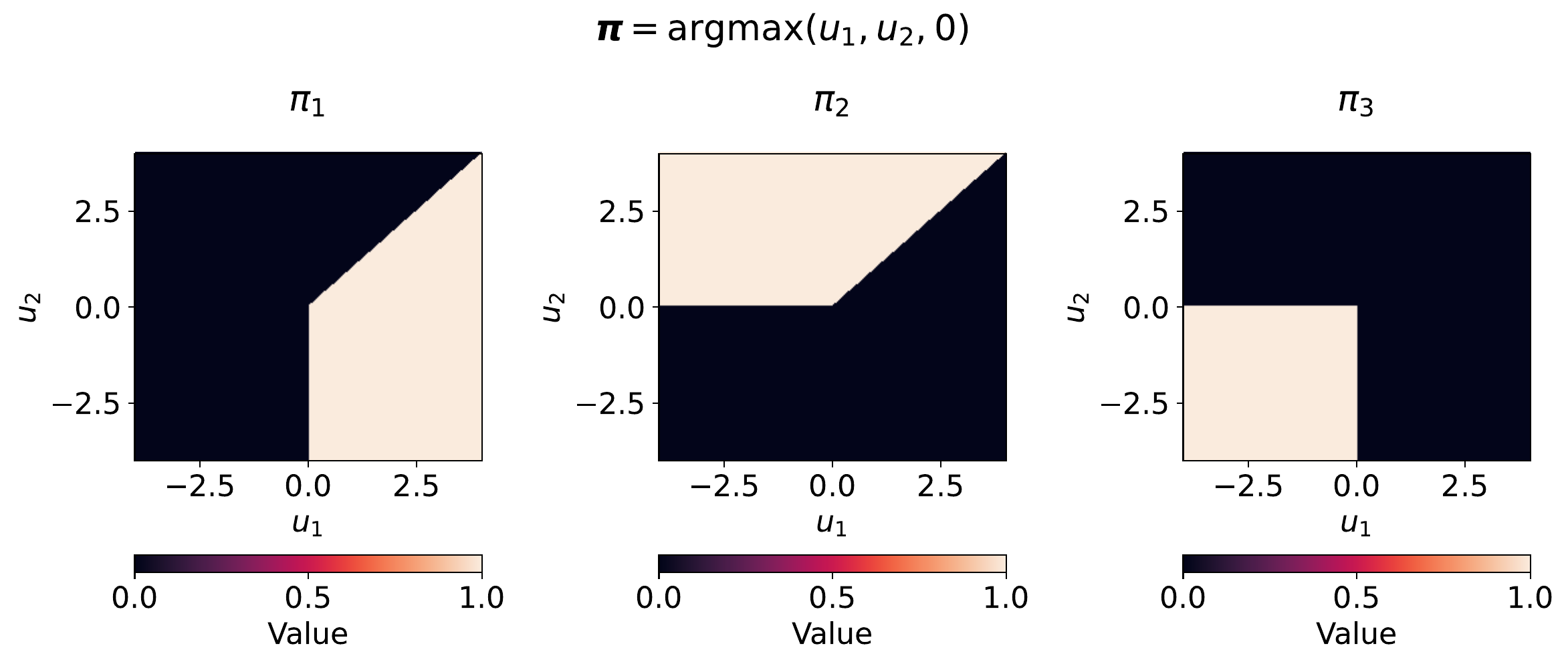
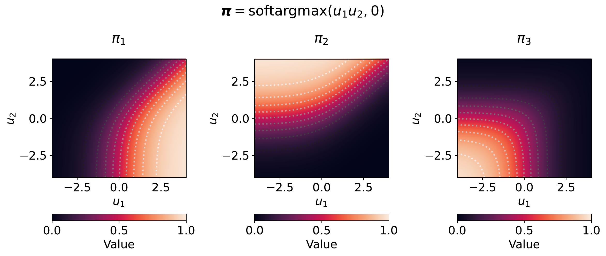
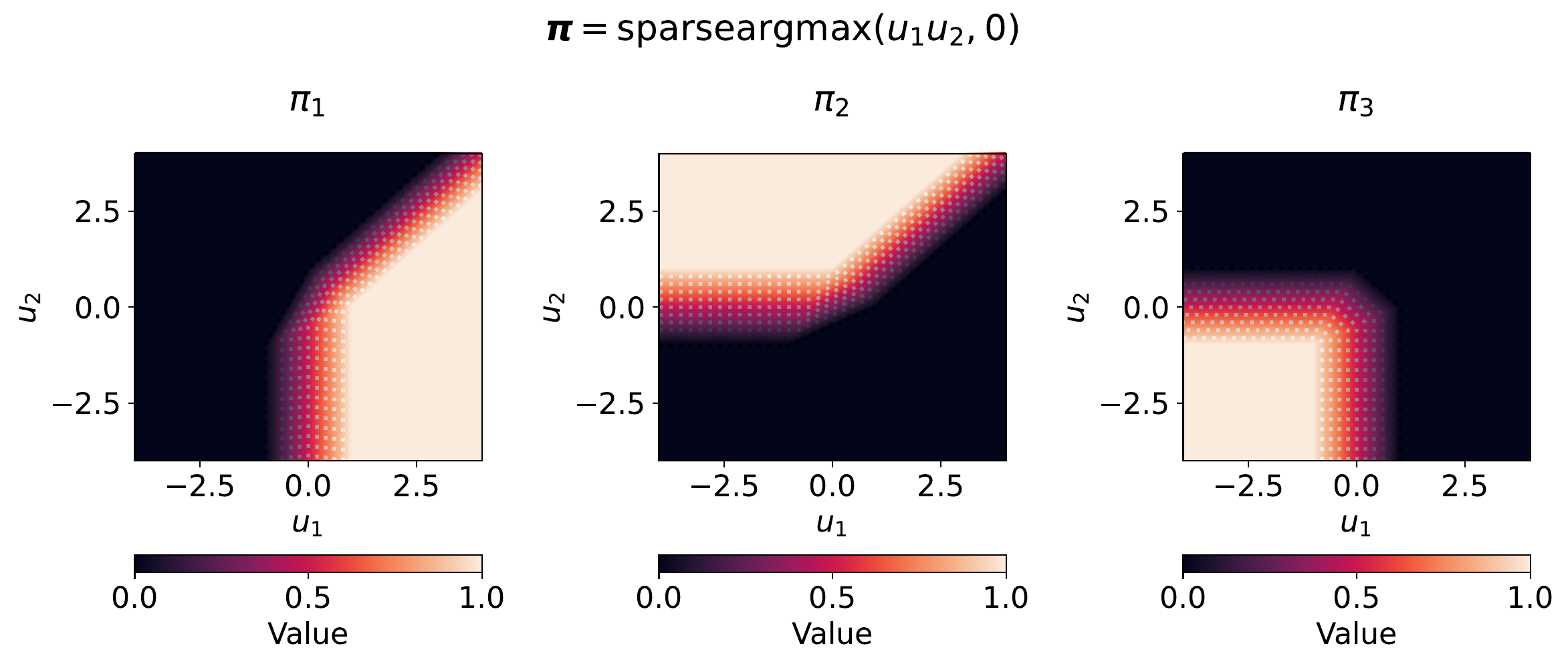
Figure 13.9: Values of , , and for , when varying and . The argmax is a piecewise constant, discontinuous function. The softargmax is a continuous and differentiable everywhere function, but it is always strictly positive and therefore dense. The sparseargmax is a continuous function and its output can be sparse, but it is only a differentiable almost everywhere function.
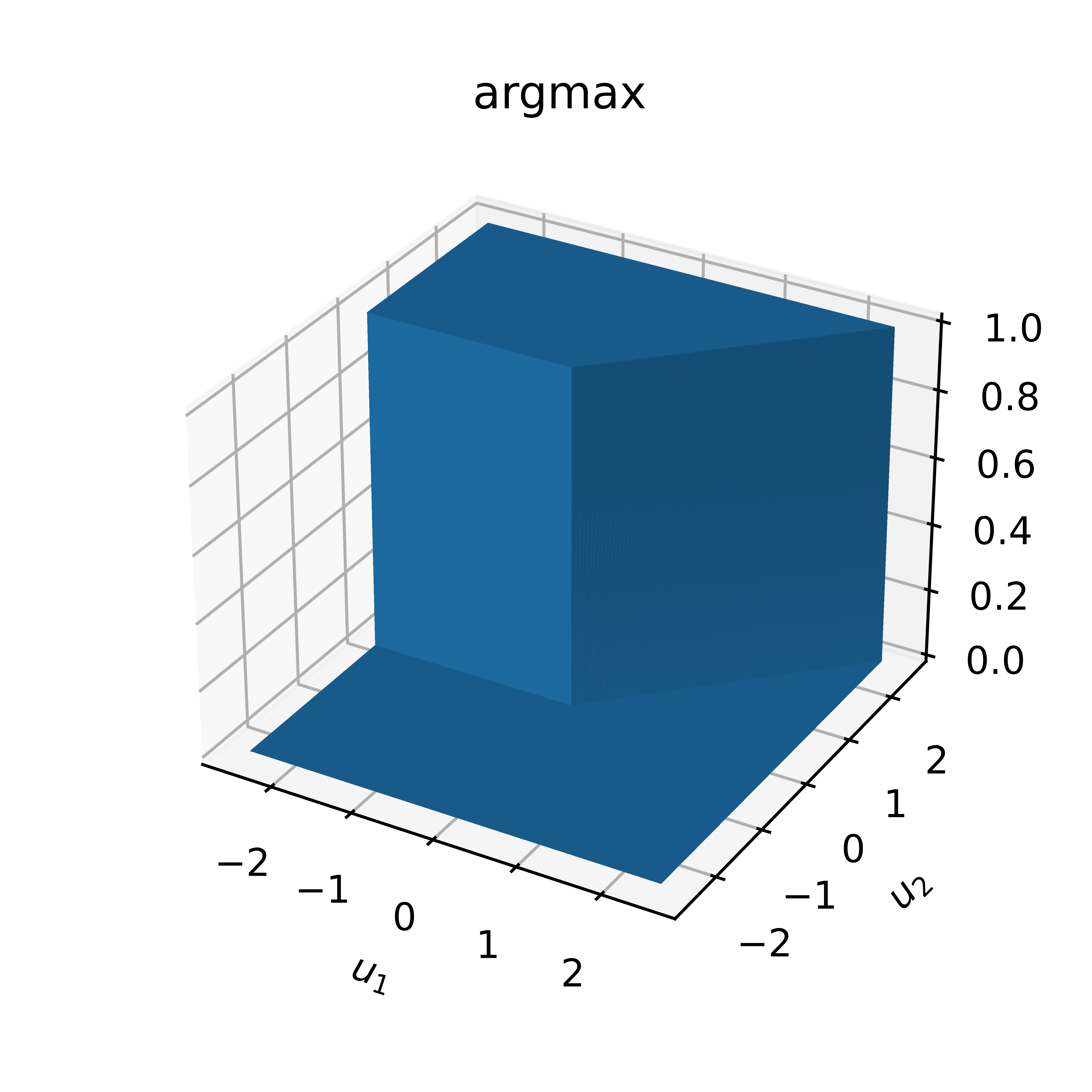
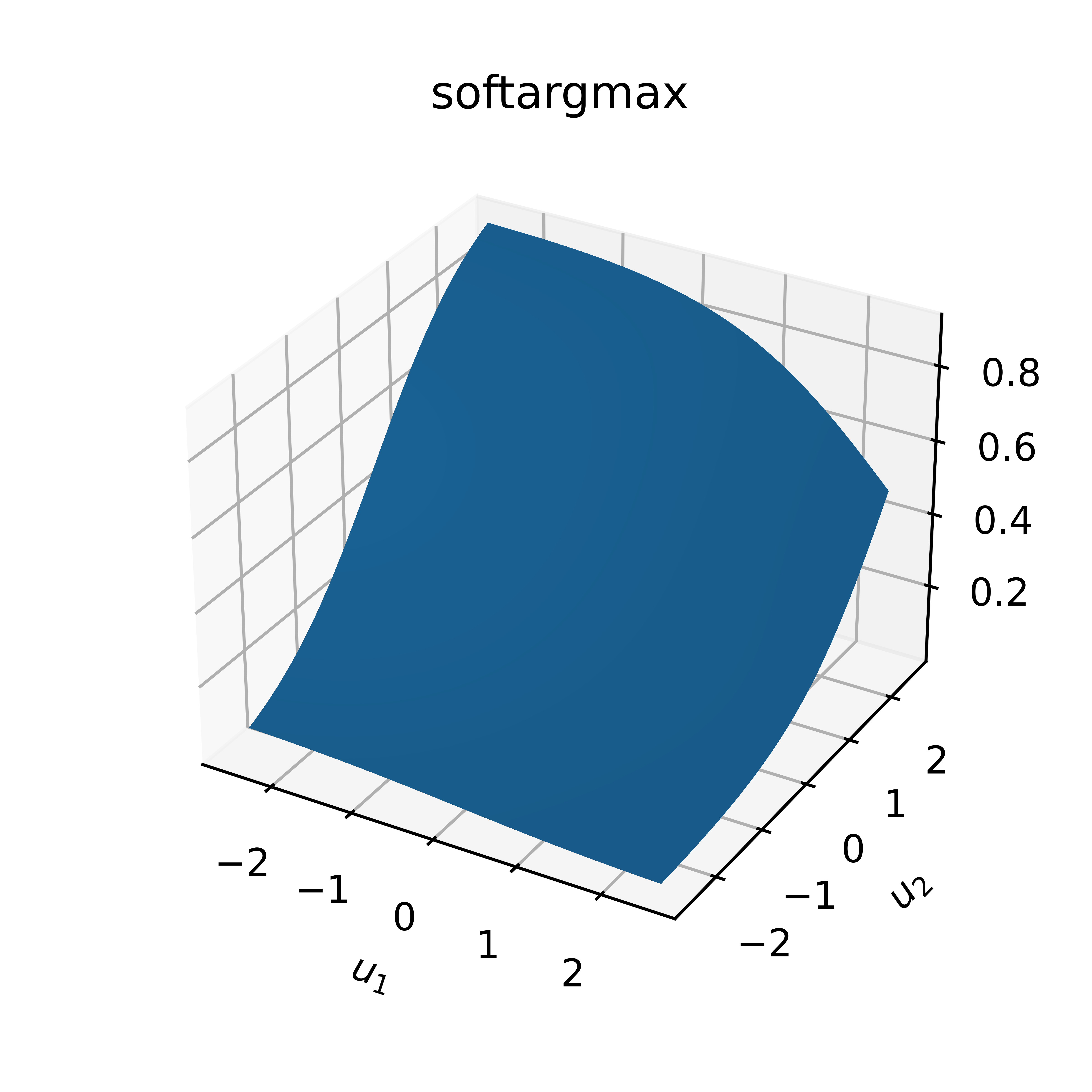
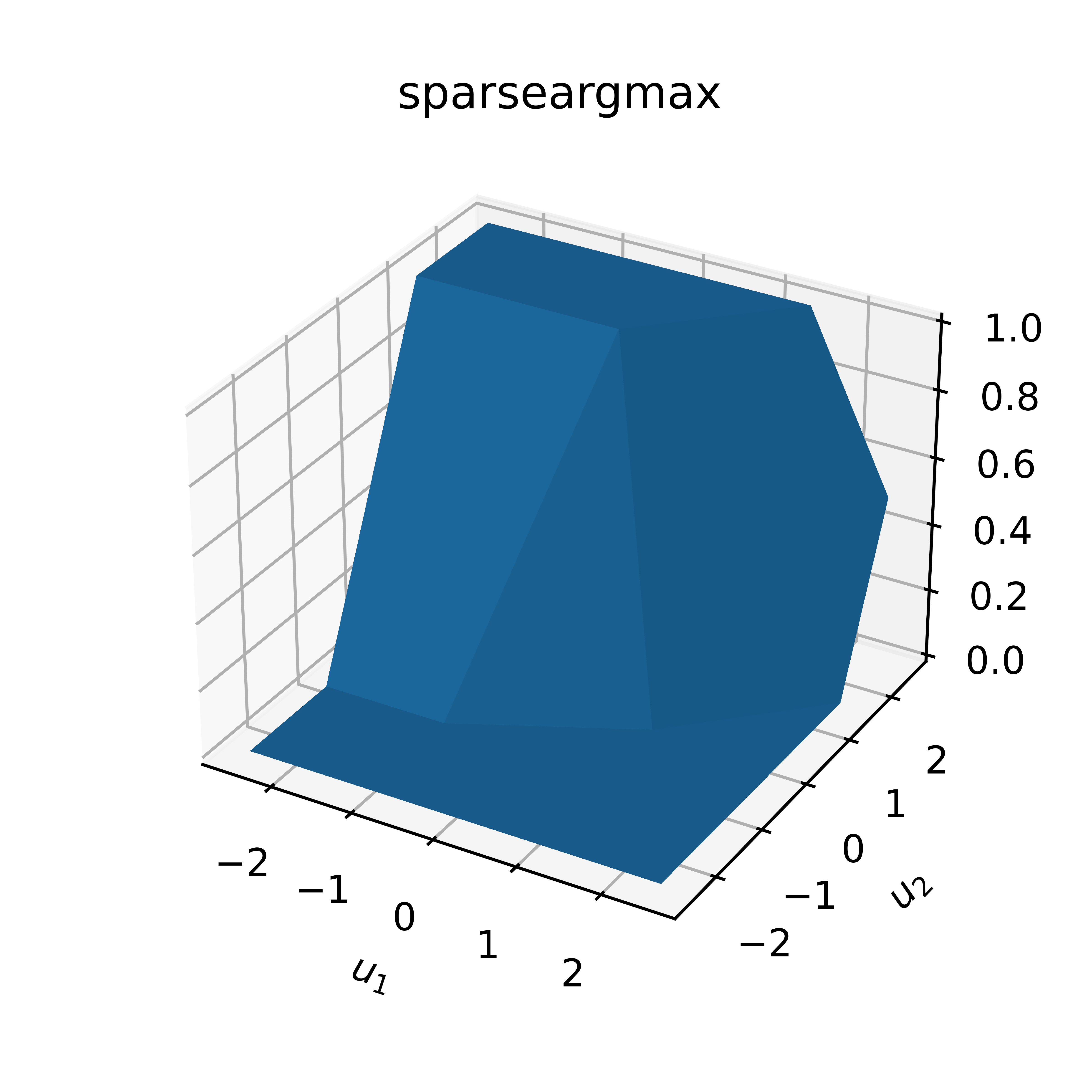
Figure 13.10: Same as Fig. 13.9 but using a 3D plot.
Relaxed argmin operators
The argmin operator can be expressed in terms of the argmax operator, Given a relaxed argmax operator , we can therefore define a relaxed argmin by We then have for all
13.8 Summary
When a function is non-differentiable (or worse, discontinuous), a reasonable approach is to replace it by its smooth approximation (or continuous relaxation).
The first approach we reviewed is infimal convolution between and primal regularization . The Moreau envelope is a special case, obtained by using .
The second approach we reviewed is regularizing the convex conjugate of with some dual regularization . We saw that the primal and dual approaches are equivalent when .
The Legendre-Fenchel transformation, a.k.a. convex conjugate, can be seen as a dual representation of a function: instead of representing by its graph for , we can represent it by the set of tangents with slope and intercept for . As its name indicates, it is convex, even if the original function is not.
We showed how to apply smoothing techniques to create smoothed ReLU functions and smoothed max operators. We also showed that taking their gradients allowed us to obtain generalized sigmoid functions and argmax operators.