Chapter 3Probabilistic learning
In this chapter, we review how to perform probabilistic learning. We also introduce exponential family distributions, as they play a key role in this book.
3.1 Probability distributions
3.1.1 Discrete probability distributions
A discrete probability distribution over a set is specified by its probability mass function (PMF) . The probability of is then defined by where denotes a random variable. When follows a distribution , we write (with some abuse of notation, we use the same letter to denote the distribution and the PMF). The expectation of , where and , is then its variance (for one-dimensional variables) is and its mode is The Kullback-Leibler (KL) divergence (also known as relative entropy) between two discrete distributions over , with associated PMFs and , is the statistical “distance” defined by
3.1.2 Continuous probability distributions
A continuous probability distribution over is specified by its probability density function (PDF) . The probability of is then The expectation, variance and KL divergence are defined analogously to the discrete setting, simply replacing with . Specifically, the expectation of is the variance is and the KL divergence is The mode is defined as the argmax of the PDF.
When , we can also define the cumulative distribution function (CDF) The probability of lying in the semi-closed interval is then
3.2 Maximum likelihood estimation
3.2.1 Negative log-likelihood
We saw that a probability distribution over is specified by , which is called the probability mass function (PMF) for discrete variables or the probability density function (PDF) for continuous variables. In practice, the true distribution generating the data is unknown and we wish to approximate it with a distribution , with parameters . Given a finite set of i.i.d. observations , how do we fit to the data? This can be done by maximizing the likelihood of the data, i.e., we seek to solve This is known as maximum likelihood estimation (MLE). Because the function is monotonically increasing, this is equivalent to minimizing the negative log-likelihood, i.e., we have
Example 3.1 (MLE for the normal distribution)
Suppose we set to the normal distribution with parameters , i.e., Then, given observations , the MLEs for and are the sample mean and the sample variance, respectively.
3.2.2 Consistency w.r.t. the Kullback-Leibler divergence
It is well-known that the MLE is consistent, in the sense of the Kullback-Leibler divergence. That is, denoting the true distribution and where then in expectation over the observations, as . This can be seen by using and the law of large numbers.
3.3 Probabilistic supervised learning
3.3.1 Conditional probability distributions
Many times in machine learning, instead of a probability for some , we wish to define a conditional probability , for some input . This can be achieved by reduction to an unconditional probability distribution, where and is a model function with model parameters . That is, rather than being a deterministic function from to , is a function from to , the set of permissible distribution parameters of the output distribution associated with the input.
We emphasize that could be a single parameter or a collection of parameters. For instance, in the Bernoulli distribution, , while in the univariate normal distribution, .
In Section 3.4 and throughout this book, we will also use the notation instead of when are the canonical parameters of an exponential family distribution.
3.3.2 Inference
The main advantage of this probabilistic approach is that our prediction model is much richer than if we just learned a function from to . We now have access to the whole distribution over possible outcomes in and can compute various statistics:
Probability: or ,
Expectation: for some function ,
Variance: ,
Mode: .
We now review probability distributions useful for binary classification, multiclass classification, regression, multivariate regression, and integer regression. In the following, to make the notation more lightweight, we omit the dependence on .
3.3.3 Binary classification
For binary outcomes, where , we can use a Bernoulli distribution with parameter When a random variable is distributed according to a Bernoulli distribution with parameter , we write The PMF of this distribution is The Bernoulli distribution is a binomial distribution with a single trial. Since , the PMF can be rewritten as The mean is and the variance is
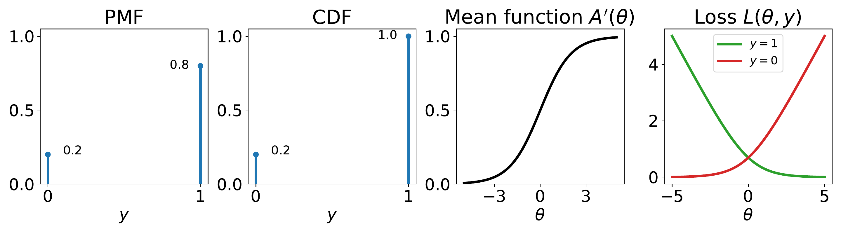
Figure 3.1: The Bernoulli distribution, whose PMF and CDF are here illustrated with parameter . Its mean function is , where is for instance the output of a neural network. The negative log-likelihood leads to the logistic loss, . The loss curve is shown for .
Parameterization using a sigmoid
Since the parameter of a Bernoulli distribution needs to belong to , we typically use a sigmoid function (Section 4.4.3), such as a logistic function as the output layer: where is for example a neural network and When is linear in , this is known as binary logistic regression.
Remark 3.1 (Link with the logistic distribution)
The logistic distribution with mean and scale parameters and is a continuous probability distribution with PDF where If a random variable follows a logistic distribution with parameters and , we write . The CDF of is Therefore, if and then Here, can be interpreted as a latent continuous variable and as a threshold.
3.3.4 Multiclass classification
For categorical outcomes with possible choices, where , we can use a categorical distribution with parameters where we define the probability simplex i.e., the set of valid discrete probability distributions. When follows a categorical distribution with parameter , we write The PMF of the categorical distribution is where is the standard basis vector for the coordinate .
Since is a categorical variable, it does not make sense to compute the expectation of but we can compute that of , Therefore, as was also the case for the Bernoulli distribution, the mean and the probability distribution (represented by the vector ) are the same in this case.
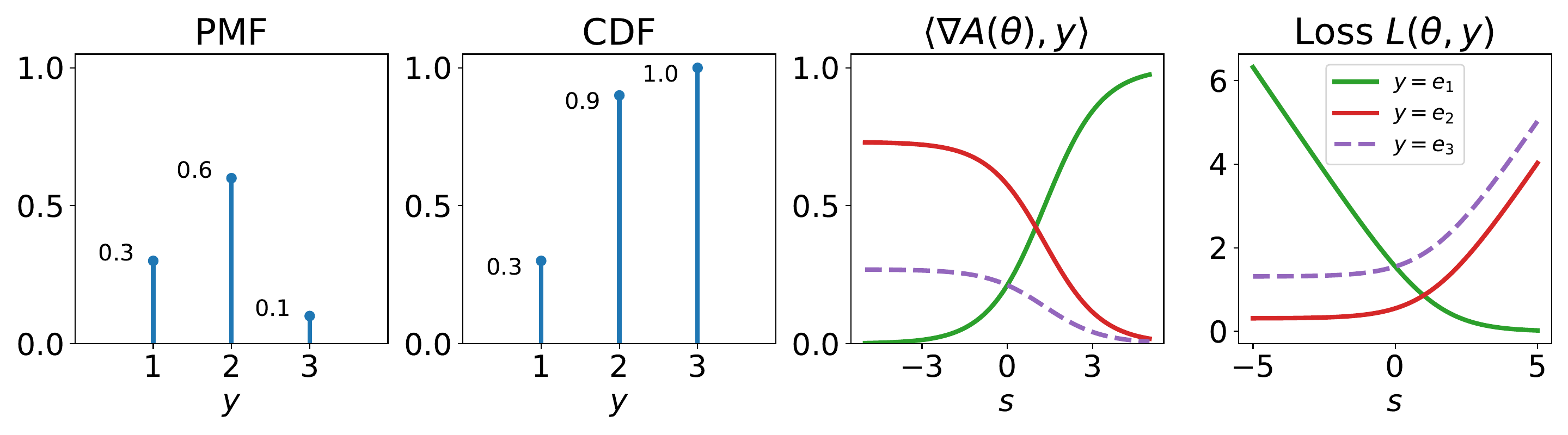
Figure 3.2: The categorical distribution, whose PMF and CDF are here illustrated with parameter . Its mean function is , where is for instance the output of a neural network. Here, for illustration purpose, we choose to set and vary only . Since the mean function belongs to , we choose to display , for . The negative log-likelihood leads to the logistic loss, . The loss curve is shown for , again with and varying .
Parameterization using a softargmax
Since the parameter vector of a categorical distribution needs to belong to , we typically use a softargmax as the output layer: where is for example a neural network and The output of the softargmax is in the relative interior of , . That is, the produced probabilities are always strictly positive. The categorical distribution is a multinomial distribution with a single trial. When is linear in , this is therefore known as multiclass or multinomial logistic regression, though strictly speaking a multinomial distribution could use more than one trial.
3.3.5 Regression
For real outcomes, where , we can use, among other choices, a normal distribution with parameters where is the mean parameter and is the standard deviation parameter. When follows a normal distribution with parameters , we write The PDF is The expectation is One advantage of the probabilistic perspective is that we are not limited to predicting the mean. We can also compute the CDF where we used the error function This function is available in most scientific computing libraries, such as SciPy (Virtanen et al., 2020). We can also write where is the CDF of the standard Gaussian distribution (with zero mean and unit variance). From the CDF, we also easily obtain
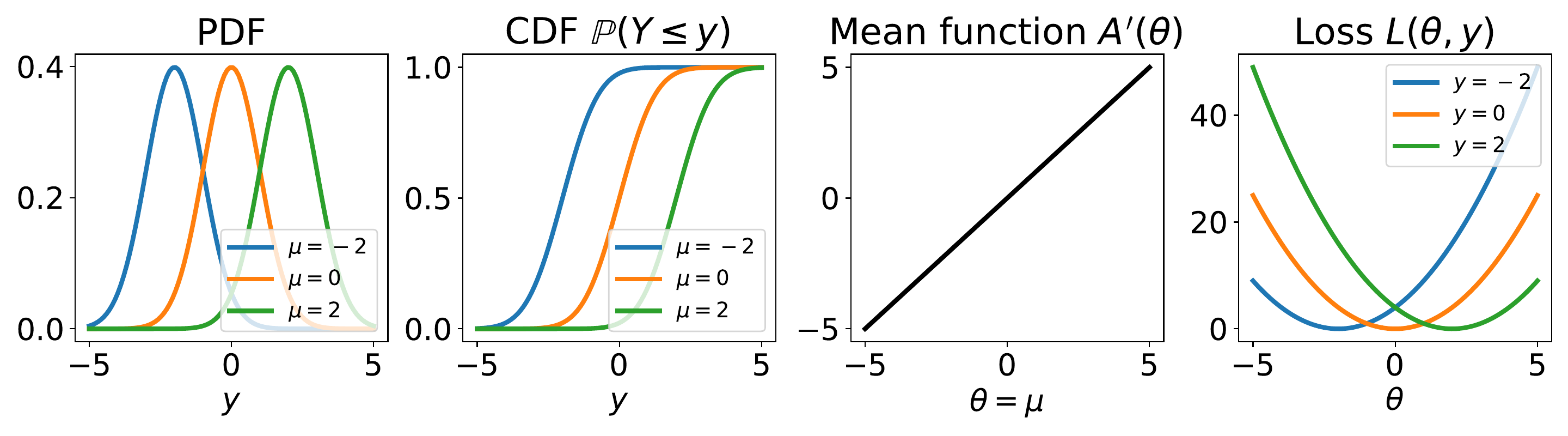
Figure 3.3: The Gaussian distribution, with mean parameter and variance . Its mean function is , where is for instance the output of a neural network. The negative log-likelihood leads to the squared loss, . The loss curve is shown for .
Parameterization
Typically, in regression, the mean is output by a model, while the standard deviation is kept fixed (typically set to ). Since is unconstrained, we can simply set where is for example a neural network. That is, the output of is the mean of the distribution, We can also use to predict or , as shown above.
3.3.6 Multivariate regression
More generally, for multivariate outcomes, where , we can use a multivariate normal distribution with parameters where is the mean and is the covariance matrix. When follows a multivariate normal distribution with parameters , we write The PDF is Using a diagonal covariance matrix is equivalent to using independent normal distributions for each , for . The expectation is
Parameterization
Typically, in multivariate regression, the mean is output by a model, while the covariance matrix is kept fixed (typically set to the identity matrix). Since is again unconstrained, we can simply set More generally, we can parametrize the function so as to output both the mean and the covariance matrix , i.e., The function must be designed such that is symmetric and positive semi-definite. This is easy to achieve for instance by parametrizing for some matrix .
3.3.7 Integer regression
For integer outcomes, where , we can use, among other choices, a Poisson distribution with mean parameter . When follows a Poisson distribution with parameter , we write The PMF is It is the probability of events occurring in an interval of time. The Poisson distribution is frequently used when there is a large number of possible events, each of which is rare.
The CDF is The Poisson distribution implies that the index of dispersion (the ratio between variance and mean) is , since When this assumption is inappropriate, one can use generalized Poisson distributions (Satterthwaite, 1942).
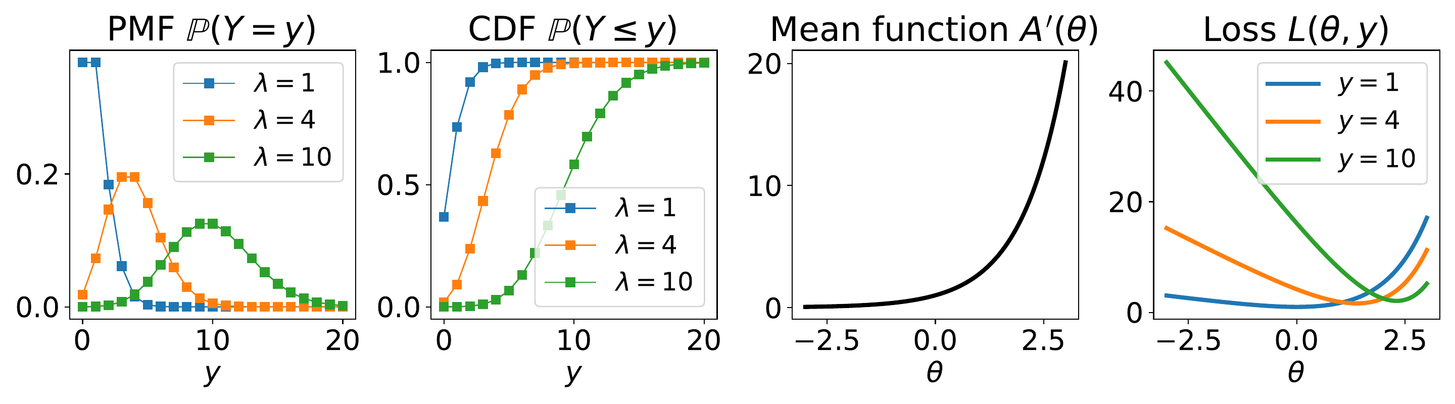
Figure 3.4: The Poisson distribution, with mean parameter . For the PMF and the CDF, the lines between markers are shown for visual aid: the Poisson distribution does not assign probability mass to non-integer values. Its mean function is , where is for instance the output of a neural network. The negative log-likelihood leads to the Poisson loss, , which is a convex function of . The loss curve is shown for .
Parameterization using an exponential
Since the parameter of a Poisson distribution needs to be strictly positive, we typically use an exponential function as output layer: where .
3.3.8 Loss functions
We now discuss how to learn the model parameters from input-output pairs .
Deterministic vs. probabilistic approaches
In a deterministic approach, if we used a mapping , we could formulate an objective function of the form where is a loss function. Unfortunately, would be typically discontinuous if is a discrete output space (as is the case in classification), making optimization difficult.
In contrast, in the probabilistic approach, we use a mapping to distribution parameters, and we can formulate an objective of the form where . This is typically a continuous objective, since is typically a continuous set and varies continuously w.r.t. even if is a distribution over a discrete set . In other words, the probabilistic approach is not only powerful for the inference it allows us to do (probability, expectation, variance, mode), but also because it allows us to formulate a continuous and typically differentiable objective function!
This is summarized in Fig. 3.5.
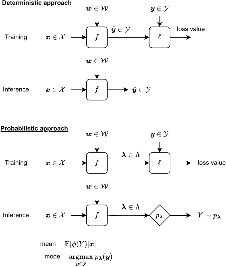
Figure 3.5: Summary of deterministic vs. probabilistic approaches.
Negative log-likelihood
In the conditional setting briefly reviewed in Section 3.3.1, we can use maximum likelihood estimation (MLE) to estimate the model parameters of . Given a set of input-output pairs , we choose the model parameters that maximize the likelihood of the data, where Again, this is equivalent to minimizing the negative log-likelihood, In the notation above, this corresponds to defining the loss function
Recovering well-known loss functions
Interestingly, MLE allows us to recover several popular loss functions.
For the Bernoulli distribution with parameter , where , we have which is the binary logistic loss function.
For the categorical distribution with parameters , where , we have which is the multiclass logistic loss function, also known as cross-entropy loss.
For the normal distribution with mean and fixed variance , we have which is, up to a constant and with unit variance, the squared loss function.
For the Poisson distribution with mean , where , we have which is the Poisson loss function. The loss function is convex w.r.t. and for .
3.4 Exponential family distributions
3.4.1 Definition
The exponential family is a class of probability distributions, whose PMF or PDF can be written in the form where are the natural or canonical parameters of the distribution. The function is known as the base measure. The function is the sufficient statistic: it holds all the information about and is used to embed in a vector space. The function is the log-partition or log-normalizer (see below for details). All the distributions we reviewed in Section 3.3 belong to the exponential family. With some abuse of notation, we use for the distribution in original form and for the distribution in exponential family form. As we will see, we can go from to and vice versa. We illustrate how to rewrite a distribution in exponential family form below.
Example 3.2 (Bernoulli distribution)
The PMF of the Bernoulli distribution with parameter equals Therefore, Bernoulli distributions belong to the exponential family, with natural parameter . Conversely, we have .
We rewrite the previously-described distributions in exponential family form in Table 3.1. This list is non-exhaustive: there are many more distributions in the exponential family! (Barndorff-Nielsen, 2014)
Table 3.1: Examples of distributions in the exponential family.
| Bernoulli | Categorical | |
|---|---|---|
| 1 | 1 | |
| Normal (location only) | Normal (location-scale) | |
| Multivariate normal | Poisson | |
3.4.2 The log-partition function
We focus our discussion in this section on discrete variables for simplicity. However, the results stated in this section also hold for continuous variables (Wainwright and Jordan, 2008). The log-partition function is the logarithm of the distribution’s normalization factor, We denote the set of valid parameters We can conveniently rewrite as where we defined the affine map Since is the composition of , a convex function, and of , an affine map, we immediately obtain the following proposition.
Proposition 3.1 (Convexity of the log-partition)
is a convex function.
A major property of the log-partition function is that its gradient coincides with the expectation of according to .
Proposition 3.2 (Gradient of the log-partition)
Proof
The result follows directly from ◻
The gradient is therefore often called the mean function. The set of achievable means is defined by where is the convex hull of and is the set of valid probability distributions over .
Similarly, the Hessian coincides with the covariance matrix of according to (Wainwright and Jordan, 2008, 3).
When the exponential family is minimal, which means that the parameters uniquely identify the distribution, it is known that is a one-to-one mapping from to . That is, and .
3.4.3 Maximum entropy principle
Suppose we observe the empirical mean of some observations . How do we find a probability distribution achieving this mean? Clearly, such a distribution may not be unique. One way to choose among all possible distributions is by using the maximum entropy principle. Let us define the Shannon entropy by for discrete variables and by for continuous variables. This captures the level of “uncertainty” in , i.e., it is maximized when the distribution is uniform. Then, the maximum entropy distribution satisfying the first-order moment condition (i.e., whose expectation matches the empirical mean) is It can be shown that the maximum entropy distribution is necessarily in the exponential family with sufficient statistic defined by and its canonical parameters coincide with the Lagrange multipliers of the above constraint (Wainwright and Jordan, 2008, Section 3.1).
3.4.4 Maximum likelihood estimation
As in Section 3.2, to fit the parameters of an exponential family distribution to some i.i.d. observations , we can use the MLE principle, i.e., Fortunately, for exponential family distributions, the log probability/density enjoys a particularly simple form.
Proposition 3.3 (Negative log-likelihood)
The negative log-likelihood of an exponential family distribution is Its gradient is and its Hessian is which is independent of .
It follows from Proposition 3.1 that is convex. Interestingly, we see that the gradient is the residual between the expectation of according to the model and the observed . Therefore, the negative log-likelihood of an exponential family distribution can be seen as performing first moment matching.
3.4.5 Probabilistic learning with exponential families
In the supervised probabilistic learning setting, we wish to estimate a conditional distribution of the form . Given a model function , such as a neural network, a common approach for defining such a conditional distribution is by reduction to the unconditional setting, In other words, the role of is to produce the parameters of given some input . It is a function from to . Note that must be designed such that it produces an output in Many times, will be the entire but this is not always the case. For instance, as we previously discussed, for a multivariate normal distribution, where , we need to ensure that is a positive semidefinite matrix.
Training
Given input-output pairs , we then seek to find the parameters of by minimizing the negative log-likelihood where . While is a convex function of for exponential family distributions, we emphasize that is typically a nonconvex function of , when is a nonlinear function, such as a neural network.
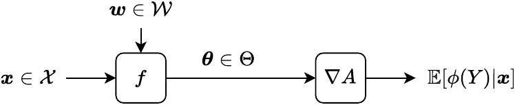
Figure 3.6: Generalized linear models.
Inference
Once we have found by minimizing the objective function above, there are several possible strategies to perform inference for a new input .
Expectation. When the goal is to compute the expectation of , we can use . That is, we compute the distribution parameters associated with by and then we compute the mean by . When is linear in , the composition is called a generalized linear model. This is illustrated in Fig. 3.6.
Probability. When the goal is to compute the probability of a certain , we can compute the distribution parameters associated with by and then we can compute . In the particular case of the categorical distribution (of which the Bernoulli distribution is a special case), we point out again that the mean and the probability vector coincide:
Other statistics. When the goal is to compute other quantities, such as the variance or the CDF, we can convert the natural parameters to the original distribution parameters (see Table 3.1 for examples). Then, we can use established formulas for the distribution in original form, to compute the desired quantities.
3.5 Summary
We reviewed discrete and continuous probability distributions.
We saw how to fit distribution parameters to data using the maximum likelihood estimation (MLE) principle and saw its connection with the Kullback-Leibler divergence.
Instead of designing a model function from the input space to the output space , we saw that we can perform probabilistic supervised learning by designing a model function from to distribution parameters .
Leveraging the so-obtained parametric conditional distribution then allowed us to compute, not only output probabilities, but also various statistics such as the mean and the variance of the outputs.
We reviewed the exponential family, a principled generalization of numerous distributions, which we saw is tightly connected with the maximum entropy principle.
Importantly, the approaches described in this chapter produce perfectly valid computation graphs, meaning that we can combine them with neural networks and we can use automatic differentiation, to compute their derivatives.