Part I Fundamentals

Chapter 2Differentiation

In this chapter, we review key differentiation concepts. In particular, we emphasize the fundamental role played by linear maps.

2.1 Univariate functions

2.1.1 Derivatives

To study functions, we need to capture their infinitesimal variations around points as defined by the notion of limit.

Definition 2.1 (Limit)

We say that $c \in \RR$ is the limit of $f \colon \RR \to \RR$ as $v \in \RR$ approaches $w \in \RR$ , denoted $\lim_{v \rightarrow w} f(v) = c,$ if, for any $\varepsilon > 0$ , there exists $R > 0$ such that for any $v \in \RR$ satisfying $0<|v -w| \leq R$ , we have $|f(v) - c| \leq \varepsilon$ .

We can also write $f(v) \to c$ as $v \to w$ . Limits are preserved under additions and multiplications. Namely, if $\lim_{v \rightarrow w} f(v) = c$ and $\lim_{v \rightarrow w} g(v) = d$ , then denoting $(af + bg)(w) \coloneqq af(w) + bg(w)$ for any $a, b \in \RR$ and $(fg)(w) \coloneqq f(w) g(w)$ , we have by definition of the limit, $\lim_{v \rightarrow w} (af + bg)(v) = ac + bd$ and $\lim_{v \rightarrow w} (fg)(v) = cd$ . The preservation of the limit under addition and multiplication by a scalar is generally referred to as the linearity of the limit, a property that many definitions in the sequel inherit.

With the notion of limit, we can already delineate a class of “well-behaved” functions: functions whose limit at any point equals the value of the function at that point. Functions satisfying this property are called continuous.

Definition 2.2 (Continuous function)

A function $f:\RR \rightarrow \RR$ is continuous at a point $w \in \RR$ if $\lim_{v \rightarrow w} f(v) = f(w).$ A function $f$ is said to be continuous if it is continuous at all points in its domain.

Although the notion of continuity appears to be a benign assumption, several functions commonly used in machine learning, such as the Heaviside step function (displayed in the left panel of Fig. 2.2), are not continuous and require special treatment.

Remark 2.1 (Little $o$ notation)

In the following, we will make use of Landau’s little $o$ notation. We write $g(v) = o(f(v)) \ \mbox{as} \ v \rightarrow w$ if $\lim_{v\rightarrow w} \frac{|g(v)|}{|f(v)|} = 0.$ That is, the function $f$ dominates $g$ in the limit $v \to w$ . For example, $f$ is continuous at $w$ if and only if $f(w+\delta) = f(w) + o(1) \ \mbox{as} \ \delta \rightarrow 0.$

We now explain derivatives. Consider a function $f: \RR\rightarrow \RR$ . As illustrated in Fig. 2.1, its value on an interval $[w_0, w_0+\delta]$ can be approximated by the secant between its values $f(w_0)$ and $f(w_0+\delta)$ , a linear function with slope $(f(w_0+\delta) - f(w_0))/\delta$ . In the limit of an infinitesimal variation $\delta$ around $w_0$ , the secant converges to the tangent of $f$ at $w_0$ and the resulting slope defines the derivative of $f$ at $w_0$ . The definition below formalizes this intuition.

Definition 2.3 (Derivative)

The derivative of $f:\RR \rightarrow\RR$ at $w\in \RR$ is defined as $f'(w) \coloneqq \lim_{\delta\rightarrow 0} \frac{f(w+\delta)- f(w)}{\delta}, \tag{2.1}$ provided that the limit exists. If $f'(w)$ is well-defined at a particular $w$ , we say that the function $f$ is differentiable at $w$ . If $f$ is differentiable at any $w\in \RR$ , we say that it is differentiable everywhere or differentiable for short.

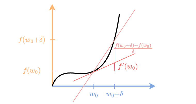
Figure 2.1: A function $f$ can be locally approximated around a point $w_0$ by a secant, a linear function $w \mapsto aw + b$ with slope $a$ and intercept $b$ , crossing $f$ at $w_0$ with value $u_0= f(w_0)$ and crossing at $w_0 + \delta$ with value $u_\delta=f(w_0+\delta)$ . Using $u_0 = a w_0 + b$ and $u_\delta = a(w_0 + \delta) + b$ , we find that its slope is $a = (f(w_0 + \delta) - f(w_0)) / \delta$ and the intercept is $b=f(w_0) -aw_0$ . The derivative $f'(w)$ of a function $f$ at a point $w_0$ is then defined as the limit of the slope $a$ when $\delta \to 0$ . It is the slope of the tangent of $f$ at $w_0$ . The value $f(w)$ of the function at $w$ can then be locally approximated around $w_0$ by $w \mapsto f'(w_0) w + f(w_0) - f'(w_0) w_0 = f(w_0) + f'(w_0)(w - w_0)$ .

If $f$ is differentiable at a given $w$ , then it is necessarily continuous at $w$ as shown in the following proposition. Non-differentiability of a continuous function at a given point $w$ is generally illustrated by a kink, as shown in Fig. 2.2.

Proposition 2.1 (Differentiability implies continuity)

If $f:\RR \rightarrow \RR$ is differentiable at $w\in \RR$ , then it is continuous at $w\in \RR$ .

Proof

In little $o$ notation, $f$ is differentiable at $w$ if there exists $f'(w) \in \RR$ , such that $f(w+\delta) = f(w) + f'(w)\delta + o(\delta) \ \mbox{as} \ \delta \rightarrow 0.$ Since $f'(w)\delta + o(\delta) = o(1)$ as $\delta \rightarrow 0$ , $f$ is continuous at $w$ . ◻

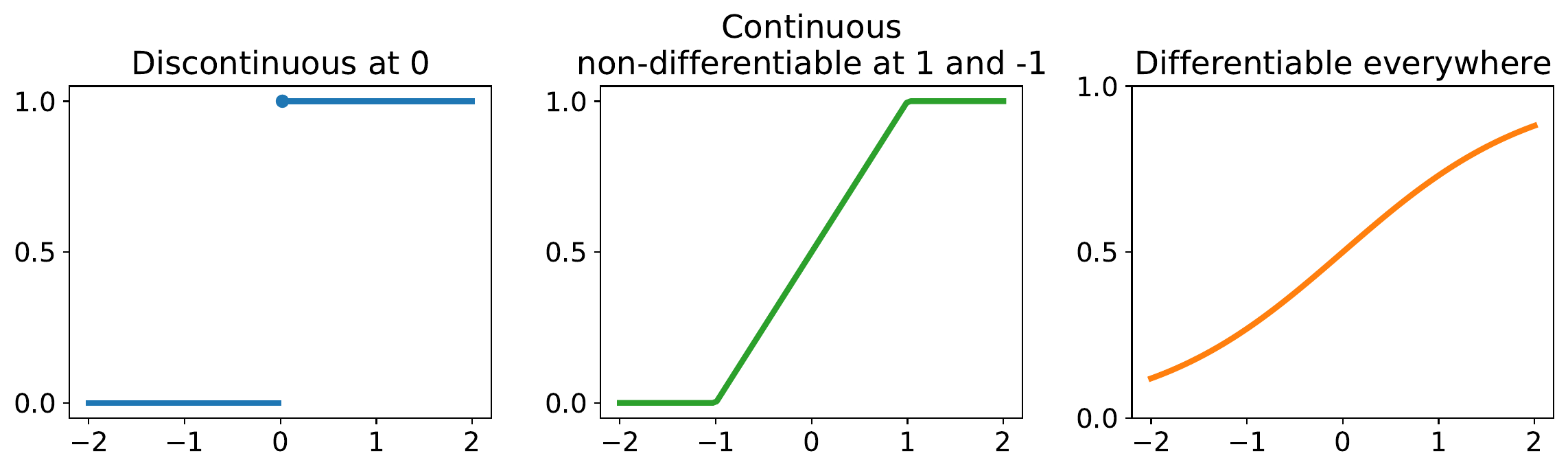
Figure 2.2: Illustration of discontinuity and non-differentiability. Left. A discontinuous function, with a jump in function value at $0$ . Center. A continuous but non-differentiable everywhere function, with kinks at $-1$ and $1$ . Right. A differentiable everywhere function.

In addition to enabling the construction of a linear approximation of $f$ in a neighborhood of $w$ , since it is the slope of the tangent of $f$ at $w$ , the derivative $f'$ informs us about the monotonicity of $f$ around $w$ . If $f'(w)$ is positive, the function is increasing around $w$ . Conversely, if $f'(w)$ is negative, the function is decreasing. Such information can be used to develop iterative algorithms such as gradient descent, which seeks to minimize $f$ by computing iterates of the form $w_{t+1}= w_t - \gamma f'(w_t)$ for $\gamma>0$ , thereby moving along descent directions of $f$ around $w_t$ .

For several elementary functions such as $w^n$ , $e^w$ , $\ln w$ , $\cos w$ or $\sin w$ , their derivatives can be obtained directly by applying the definition of the derivative in Eq. (2.1) as we now illustrate.

Example 2.1 (Derivative of power function)

Consider $f(w) = w^n$ for $w \in \RR$ , $n\in \N\setminus\{0\}$ . For any $\delta \in \RR$ , we have $\begin{align*} \frac{f(w+\delta) - f(w)}{\delta} & = \frac{(w+\delta)^n - w^n}{\delta} \\ & = \frac{\sum_{k=0}^{n} \binom{n}{k} \delta^k w^{n-k} - w^n}{\delta} \\ & = \sum_{k=1}^{n} \binom{n}{k} \delta^{k-1} w^{n-k} \\ & = \binom{n}{1} w^{n-1} + \sum_{k=2}^{n} \binom{n}{k} \delta^{k-1} w^{n-k}, \end{align*}$ where, in the second line, we used the binomial theorem. Since $\binom{n}{1} = n$ and $\lim_{\delta \rightarrow 0} \sum_{k=2}^{n} \binom{n}{k} \delta^{k-1} w^{n-k} =0$ , we get $f'(w)= n w^{n-1}$ .

Remark 2.2 (Functions on a subset $\cU$ of $\RR$ )

For simplicity, we presented the definition of the derivative for a function defined on the whole set of real numbers $\RR$ . If a function $f:\cU\rightarrow\RR$ is defined on a subset $\cU\subseteq \RR$ of the real numbers, as it is the case for $f(w)=\sqrt w$ defined on $\cU=\RR_+$ , the derivative of $f$ at $w\in \cU$ is defined by the limit in Eq. (2.1) provided that the function $f$ is well defined on a neighborhood of $w$ , that is, there exists $r>0$ such that $w+\delta \in \cU$ for any $|\delta|\leq r$ . The function $f$ is then said to be differentiable everywhere or differentiable for short if it is differentiable at any point $w$ in the interior of $\cU$ , the set of points $w\in \cU$ such that $\{w+\delta: |\delta|\leq r\} \subseteq \cU$ for $r$ sufficiently small. For points lying at the boundary of $\cU$ (such as $a$ and $b$ if $\cU=[a, b]$ ), one may define the right and left derivatives of $f$ at $a$ and $b$ , meaning that the limit is taken by approaching $a$ from the right or $b$ from the left.

2.1.2 Calculus rules

For a given $w\in \RR$ and two functions $f:\RR\rightarrow\RR$ and $g:\RR\rightarrow \RR$ , the derivative of elementary operations on $f$ and $g$ such as their sums, products or compositions can easily be derived from the definition of the derivative, under appropriate conditions on the differentiability of $f$ and $g$ at $w$ . For example, if the derivatives of $f$ and $g$ exist at $w$ , then the derivatives of their weighted sum or product exist, and satisfy the rules $\begin{align*} \forall a, b \in \RR, \ (af+bg)'(w) & = af'(w) +bg'(w) \tag{Linearity}\\ (fg)'(w) &= f'(w) g(w) + f(w)g'(w), \tag{Product rule} \end{align*}$ where $(fg)(w) \coloneqq f(w)g(w)$ . The linearity can be verified directly from the linearity of the limits. For the product rule, in little $o$ notation, we have, as $\delta\rightarrow 0$ , $\begin{align*} (fg)(w+\delta) & = (f(w) + f'(w)\delta+ o(\delta))(g(w) + g'(w)\delta + o(\delta)) \\ & = f(w)g(w) + f'(w)g(w)\delta + f(w)g'(w)\delta + o(\delta), \end{align*}$ hence the result.

If the derivatives of $g$ at $w$ and of $f$ at $g(w)$ exist, then the derivative of the composition $(f\circ g)(w) \coloneqq f(g(w))$ at $w$ exists and is given by $\begin{align*} \hspace{54pt} (f\circ g)'(w) = f'(g(w)) g'(w). \tag{Chain rule} \end{align*}$ We prove this result more generally in Proposition 2.2. As seen in the sequel, the linearity and the product rule can be seen as byproducts of the chain rule, making the chain rule the cornerstone of differentiation.

Consider a function that can be expressed using sums, products or compositions of elementary functions, such as $f(w) \coloneqq e^w\ln w+\cos w^2$ . Its derivative can be computed by applying the aforementioned rules on the decomposition of $f$ into elementary operations and functions.

Example 2.2 (Applying rules of differentiation)

Consider $f(w) \coloneqq e^w\ln w+\cos w^2$ . The derivative of $f$ at $w>0$ can be computed step by step as follows, denoting $\sqfn(w) \coloneqq w^2$ , $\begin{align*} \hspace*{-20pt} f'(w) & = (\exp \cdot \ln)'(w) + (\cos \circ \sqfn)'(w) \tag{Linearity}\\ \hspace*{-20pt} (\exp \cdot \ln)'(w) & = \exp'(w) \cdot \ln(w) + \exp(w) \cdot \ln'(w) \tag{Product rule} \\ \hspace*{-20pt} \quad (\cos \circ \sqfn)'(w) & = \cos'(\sqfn(w)) \sqfn'(w) \tag{Chain rule} \\ \hspace*{-20pt} \exp'(w) & = \exp(w), \hspace{30pt} \ln'(w) = 1/w, \tag{Elem. func.} \\ \hspace*{-20pt} \sqfn'(w) & = 2 w, \hspace{44pt} \cos'(w) =- \sin(w). \hspace{-3pt} \tag{Elem. func.} \end{align*}$ We therefore obtain that $f'(w) = e^w \ln w+ e^w/w - 2w\sin w^2$ .

Such a process is purely mechanical and lends itself to an automated procedure, which is the main idea of automatic differentiation presented in Chapter 8.

2.1.3 Leibniz’s notation

The notion of derivative was first introduced independently by Newton and Leibniz in the 18^th century (Ball, 1960). The latter considered derivatives as the quotient of infinitesimal variations. Namely, denoting $u = f(w)$ a variable depending on $w$ through $f$ , Leibniz considered the derivative of $f$ as the quotient $f' = \frac{du}{dw} \quad \mbox{with} \quad f'(w) = \left.\frac{du}{dw}\right|_w$ where $du$ and $dw$ denote infinitesimal variations of $u$ and $w$ respectively and the symbol $|_w$ denotes the evaluation of the derivative at a given point $w$ . This notation simplifies the statement of the chain rule first discovered by Leibniz (Rodriguez and Lopez Fernandez, 2010) as we have for $v = g(w)$ and $u = f(v)$ $\frac{du}{dw} = \frac{du}{dv} \cdot \frac{dv}{dw}.$ This hints that derivatives are multiplied when considering compositions. At evaluation, the chain rule in Leibniz notation recovers the formula presented above as $\left.\frac{du}{dw}\right|_w = \left.\frac{du}{dv}\right|_{g(w)} \left.\frac{dv}{dw}\right|_w = f'(g(w)) g'(w) = (f\circ g)'(w).$ The ability of Leibniz’s notation to capture the chain rule as a mere product of quotients made it popular throughout the centuries, especially in mechanics (Ball, 1960). The rationale behind Leibniz’s notation, the concept of “infinitesimal variations”, was questioned by later mathematicians for its potential logical issues (Ball, 1960). The notation $f'(w)$ first introduced by Euler and further popularized by Lagrange (Cajori, 1993) has then taken over in numerous mathematical textbooks. The concept of infinitesimal variations has been rigorously defined by using the set of hyperreal numbers. They extend the set of real numbers by considering each number as a sum of a non-infinitesimal part and an infinitesimal part (Hewitt, 1948). The formalism of infinitesimal variations further underlies the development of automatic differentiation algorithms through the concept of dual numbers.

2.2 Multivariate functions

2.2.1 Directional derivatives

Let us now consider a function $f:\RR^P \rightarrow \RR$ with multi-dimensional input $\w \coloneqq (w_1, \ldots, w_P) \in \RR^P$ . The most important example in machine learning is a function which, to the parameters $\w \in \RR^P$ of a neural network, associates a loss value in $\RR$ . Variations of $f$ need to be defined along specific directions, such as the variation $f(\w+\delta\v) {-}f(\w)$ of $f$ around $\w \in \RR^P$ in the direction $\v \in \RR^P$ by an amount $\delta>0$ . This consideration naturally leads to the definition of the directional derivative.

Definition 2.4 (Directional derivative)

The directional derivative of $f$ at $\w$ in the direction $\v$ is given by $\partial f(\w)[\v] \coloneqq \lim_{\delta \rightarrow 0} \frac{f(\w+ \delta \v) - f(\w)}{\delta},$ provided that the limit exists.

We use the notation $[\v]$ to emphasize that, for a given input $\w$ , we can see $\v \mapsto \partial f(\w)[\v]$ as a function. This is essential to define the differentiability of $f$ (Definition 2.6) at $\w$ and to later define linear maps (Section 2.3).

One example of directional derivative consists in computing the derivative of a function $f$ at $\w$ in any of the canonical directions $\e_i \coloneqq (0, \ldots, 0, \underbrace{1}_i, 0, \ldots, 0) .$ This allows us to define the notion of partial derivatives, denoted for $i \in [P]$ $\partial_i f(\w) \coloneqq \partial f(\w)[\ev_i] = \lim_{\delta \rightarrow 0} \frac{f(\w+ \delta \e_i) - f(\w)}{\delta}.$ This is also denoted in Leibniz’s notation as $\partial_i f(\w) = \frac{\partial f(\w)}{\partial w_i}$ or $\partial_i f(\w) = \partial_{w_i} f(\w)$ . By moving along only the $i$ ^th coordinate of the function, the partial derivative is akin to differentiating the function $\omega_i \mapsto f(w_1, \ldots, \omega_i, \ldots, w_P)$ around $\omega_i$ , letting all other coordinates fixed at their values $w_i$ .

2.2.2 Gradients

We now introduce the gradient vector, which gathers the partial derivatives. We first recall the definitions of linear map and linear form.

Definition 2.5 (Linear map, linear form)

A function $l: \RR^P \rightarrow \RR^M$ is a linear map if for any $a_1, a_2 \in \RR$ , $\v_1, \v_2 \in \RR^D$ , $l[a_1 \v_1 + a_2 \v_2] = a_1 l[\v_1] + a_2 l[\v_2].$ A linear map with values in $\RR$ , $l: \RR^P \rightarrow \RR$ , is called a linear form.

Linearity plays a crucial role in the differentiability of a function.

Definition 2.6 (Differentiability, single-output case)

A function $f: \RR^P \rightarrow \RR$ is differentiable at $\w\in \RR^P$ if its directional derivative is defined along any direction, is linear in any direction $\v$ , and if $\lim_{\|\v\|_2 \rightarrow 0} \frac{|f(\w+ \v) - f(\w) - \partial f(\w)[\v]|}{\|\v\|_2} = 0,$ where $\|\v\|_2 \coloneqq \sqrt{\langle \v, \v \rangle}$ .

We can now introduce the gradient.

Definition 2.7 (Gradient)

The gradient of a differentiable function $f: \RR^P \rightarrow \RR$ at a point $\w \in \RR^P$ is defined as the vector of partial derivatives $\nabla f(\w) \coloneqq \begin{pmatrix} \partial_1 f(\w) \\ \vdots \\ \partial_P f(\w) \end{pmatrix} = \begin{pmatrix} \partial f(\w)[\e_1] \\ \vdots \\ \partial f(\w)[\e_P] \end{pmatrix} \in \RR^P.$ By linearity, the directional derivative of $f$ at $\w$ in the direction $\v=\sum_{i=1}^P v_i \ev_i$ is then given by $\hspace{-1ex}\partial f(\w)[\v] = \sum_{i=1}^P v_i \partial f(\w)[\ev_i] = \langle \v, \nabla f(\w)\rangle \in \RR.$

Here, $\langle \cdot, \cdot \rangle$ denotes the inner product. We provide its definition in Euclidean spaces in Section 2.3.2.

In the definition above, the fact that the gradient can be used to compute the directional derivative is a mere consequence of the linearity of $\partial f(\w)[\v]$ w.r.t. $\v$ . However, in more abstract cases presented in later sections, the gradient is defined directly through this property.

As a simple example, any linear function of the form $f(\w) = \langle \a, \w \rangle = \sum_{i=1}^P a_i w_i$ is differentiable as we have $(\langle \a, \w+\v \rangle - \langle \a, \w \rangle - \langle \a, \v \rangle)/\|\v\|_2 = 0$ for any $\v$ and in particular for $\|\v\| \rightarrow 0$ . Moreover, its gradient is naturally given by $\nabla f(\w) = \a$ .

More generally, to show that a function is differentiable and find its gradient, one approach is to approximate $f(\w + \v)$ around $\v = \zeros$ . If we can find a vector $\g$ such that $f(\w+\v) = f(\w) + \langle \g, \v\rangle + o(\|\v\|_2),$ then $f$ is differentiable at $\w$ , since $\langle \g, \cdot \rangle$ is linear. Moreover, $\g$ is then the gradient of $f$ at $\w$ .

Remark 2.3 (Gateaux and Fréchet differentiability)

Multiple definitions of differentiability exist. The one presented in Definition 2.6 is that of Fréchet differentiable functions. Alternatively, if $f:\RR^P \rightarrow \RR$ has well-defined directional derivatives along any direction then the function is Gateaux differentiable. Note that the existence of directional derivatives in any direction is not a sufficient condition for the function to be differentiable. In other words, any Fréchet differentiable function is Gateaux differentiable, but the converse is not true. As a counter-example, one can verify that the function $f(x_1, x_2) \coloneqq x_1^3/(x_1^2 + x_2^2)$ is Gateaux differentiable at $0$ but not (Fréchet) differentiable at $0$ (because the directional derivative at 0 is not linear).

Some authors also require Gateaux differentiable functions to have linear directional derivatives along any direction. These are still not Fréchet differentiable functions. Indeed, the limit in Definition 2.6 is over any vectors tending to $0$ (potentially in a pathological way), while directional derivatives look at such limits uniquely in terms of a single direction.

In the remainder of this chapter, all definitions of differentiability are in terms of Fréchet differentiability.

The next example illustrates how to compute the gradient of the logistic loss and validates its differentiability.

Example 2.3 (Gradient of logistic loss)

Consider the logistic loss $\ell(\thetav, \y) \coloneqq - \langle \y, \thetav \rangle + \log \sum_{i=1}^M e^{\theta_i}$ , that measures the prediction error of the logits $\thetav \in \RR^M$ w.r.t. the correct label $\y \in \{\ev_1, \dots, \ev_M\}$ . Let us compute the gradient of this loss w.r.t. $\thetav$ for fixed $\y$ , i.e., we want to compute the gradient of $f(\thetav) \coloneqq \ell(\thetav, \y)$ . Let us decompose $f$ as $f = l + \mathrm{logsumexp}$ with $l(\thetav) \coloneqq\langle -\y, \thetav\rangle$ and $\mathrm{logsumexp}(\thetav) \coloneqq \log \sum_{i=1}^M \exp(\theta_i),$ the log-sum-exp function. The function $l$ is linear so differentiable with gradient $\nabla l(\thetav) = -\y$ . We therefore focus on $\mathrm{logsumexp}$ . Denoting $\exp(\thetav) = (\exp(\theta_1), \ldots, \exp(\theta_M))$ , using that $\exp(x) = 1 + x + o(x)$ , $\log(1+ x) = x + o(x)$ , and denoting $\odot$ the elementwise product, we get $\begin{align*} \mathrm{logsumexp}(\thetav + \v) & = \log\left(\langle \exp(\thetav + \v), \ones \rangle\right) \\ & = \log\left(\langle \exp(\thetav) \odot \exp(\v), \ones\rangle\right) \\ & = \log\left(\langle \exp(\thetav) \odot (\ones + \v + o(\|\v\|_2)), \ones\rangle\right) \\ & = \log\left(\langle \exp(\thetav), \ones\rangle + \langle \exp(\thetav), \v \rangle + o(\|\v\|_2)\right)\\ & = \log\left(\langle \exp(\thetav), \ones\rangle \right) + \left\langle \frac{\exp(\thetav)}{\langle \exp(\thetav), \ones\rangle} , \v\right\rangle + o(\|\v\|_2). \end{align*}$ The above decomposition of $\mathrm{logsumexp}(\thetav + \v)$ shows that it is differentiable, and that $\nabla \mathrm{logsumexp}(\thetav) = \softargmax(\thetav)$ , where $\begin{align*} \softargmax(\thetav) & \coloneqq \left(e^{\theta_1}/\left(\sum_{j=1}^{M}e^{\theta_j}\right), \ldots, e^{\theta_M}/\left(\sum_{j=1}^M e^{\theta_j}\right)\right). \end{align*}$ Overall, we get that $\nabla f(\thetav) = -\y + \mathrm{softargmax}(\thetav)$ .

Linearity of gradients

The notion of differentiability for multi-input functions naturally inherits from the linearity of derivatives for single-input functions. For any $u_1, \ldots, u_M \in \RR$ and any multi-input functions $f_1, \ldots, f_M$ differentiable at $\w$ , the function $u_1 f_1 + \ldots + u_M f_M$ is differentiable at $\w$ and its gradient is $\nabla (u_1 f_1 + \ldots + u_M f_M)(\w) = u_1 \nabla f_1(\w) + \ldots + u_M \nabla f_M(\w).$

Why is the gradient useful?

When $f$ is differentiable, we say that $\v$ is an ascent direction of $f$ from $\w$ if $\langle \v, \nabla f(\w) \rangle > 0.$ Conversely, we say that $\v$ is a descent direction of $f$ from $\w$ if $\langle \v, \nabla f(\w) \rangle < 0.$ Using this definition, the gradient leads to the steepest ascent direction of $f$ from $\w$ . To see why, we note that $\begin{aligned} \argmax_{\v\in \RR^P, \|\v\|_2\leq 1} \langle \v, \nabla f(\w) \rangle &= \argmax_{\v\in \RR^P, \|\v\|_2\leq 1} \partial f(\w)[\v] \\ &= \nabla f(\w)/\|\nabla f(\w)\|_2, \end{aligned}$ where we assumed $\nabla f(\w) \neq \mathbf{0}$ . The gradient $\nabla f(\w)$ is orthogonal to the level set of the function (the set of points $\w$ sharing the same value $f(\w)$ ) and points towards higher values of $f$ , as illustrated in Fig. 2.3. Conversely, the negative gradient $-\nabla f(\w)$ points towards lower values of $f$ . This observation motivates the development of optimization algorithms such as gradient descent. It is based on iteratively performing the update $\w_{t+1} \coloneqq \w_t -\gamma \nabla f(\w_t)$ , for $\gamma>0$ . It therefore seeks for a minimizer of $f$ by moving along the steepest descent direction around $\w_t$ given, up to a multiplicative factor, by $-\nabla f(\w_t)$ . See also Definition 17.1 for more details.

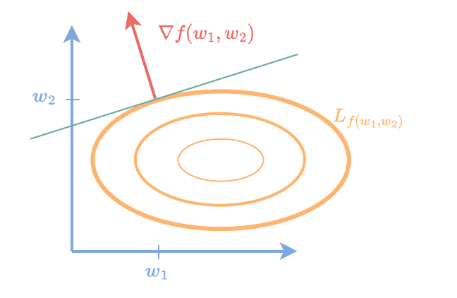
Figure 2.3: The gradient of a function $f: \RR^2\rightarrow \RR$ at $(w_1, w_2)$ is the normal vector to the tangent space of the level set $L_{f(w_1, w_2)} = \{(w_1', w_2'): f(w_1', w_2') = f(w_1, w_2)\}$ and points towards points with higher function values.

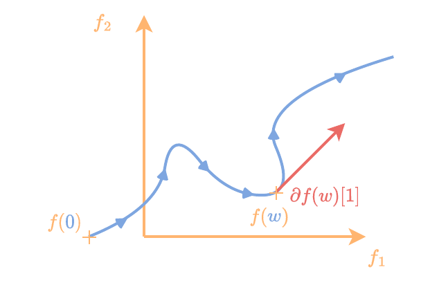
Figure 2.4: The directional derivative of a parametric curve $f:\RR \rightarrow\RR^2$ at $w$ is the tangent to the curve at the point $f(w)\in \RR^2$ .

2.2.3 Jacobians

Let us now consider a multi-output function $f:\RR^P \rightarrow \RR^M$ defined by $f(\w) \coloneqq (f_1(\w), \dots, f_M(\w))$ , where $f_j \colon \RR^P \to \RR$ . A typical example in machine learning is a neural network. The notion of directional derivative can be extended to such function by defining it as the vector composed of the coordinate-wise directional derivatives: $\partial f(\w)[\v] \coloneqq \lim_{\delta \rightarrow 0} \frac{f(\w+ \delta \v) - f(\w)}{\delta} = \lim_{\delta \rightarrow 0}\begin{pmatrix} \frac{f_1(\w+ \delta \v) - f_1(\w)}{\delta}\\ \vdots\\ \frac{f_M(\w+ \delta \v) - f_M(\w)}{\delta} \end{pmatrix} \in \RR^M,$ where the limits (provided that they exist) are applied coordinate-wise. The directional derivative of $f$ in the direction $\v \in \RR^P$ is therefore the vector that gathers the directional derivative of each $f_j$ , i.e., $\partial f(\w)[\v] = (\partial f_j(\w)[\v])_{j=1}^M$ . In particular, we can define the partial derivatives of $f$ at $\w$ as the vectors $\partial_i f(\w) \coloneqq \partial f(\w)[\ev_i] = \begin{pmatrix} \partial_i f_1(\w) \\ \vdots \\ \partial_i f_M(\w) \end{pmatrix}\in \RR^M.$ As for the usual definition of the derivative, the directional derivative can provide a linear approximation of a function around a current input, as illustrated in Fig. 2.4 for a parametric curve $f:\RR \rightarrow \RR^2$ .

Just as in the single-output case, differentiability is defined not only as the existence of directional derivatives in any direction but also by the linearity in the chosen direction.

Definition 2.8 (Differentiability, multi-output case)

A function $f:\RR^P\rightarrow \RR^M$ is (Fréchet) differentiable at a point $\w \in \RR^P$ if its directional derivative is defined along any direction, is linear in any direction, and, $\lim_{\|\v\|_2 \rightarrow 0} \frac{\|f(\w+ \v) - f(\w) - \partial f(\w)[\v]\|_2}{\|\v\|_2} = 0.$

The partial derivatives of each coordinate’s function are gathered in the Jacobian matrix.

Definition 2.9 (Jacobian)

The Jacobian of a differentiable function $f:\RR^P\rightarrow \RR^M$ at $\w$ is defined as the matrix gathering partial derivatives of each coordinate’s function provided they exist, $\begin{align*} \jac f (\w) & \coloneqq \begin{pmatrix} \partial_1 f_1(\w) & \ldots & \partial_P f_1(\w) \\ \vdots & \ddots & \vdots \\ \partial_1 f_M(\w) & \ldots & \partial_P f_M(\w) \end{pmatrix} \in \RR^{M \times P}. \end{align*}$ The Jacobian can be represented by stacking columns of partial derivatives or rows of gradients, $\begin{align*} \jac f (\w) & = \begin{pmatrix} \partial_1 f(\w), \ldots, \partial_P f(\w) \end{pmatrix} = \begin{pmatrix} \nabla f_1(\w)^\top \\ \vdots \\ \nabla f_M(\w)^\top \end{pmatrix} \in \RR^{M \times P}. \end{align*}$ By linearity, the directional derivative of $f$ at $\w$ along any input direction $\v= \sum_{i=1}^P v_i\ev_i \in \RR^P$ is then given by $\partial f(\w)[\v] = \sum_{i=1}^P v_i \partial_i f(\w) = \jac f(\w) \v \in \RR^M.$

Notice that we use bold $\jac$ to indicate the Jacobian, seen as a matrix. The Jacobian matrix naturally generalizes the concepts of derivatives and gradients presented earlier. As for the single input case, to show that a function is differentiable, one approach is to approximate $f(\w+ \v)$ around $\v=\zeros$ . If we find a linear map $l$ such that $f(\w+\v) = f(\w) + l[\v] + o(\|\v\|_2),$ then $f$ is differentiable at $\w$ . Moreover, if $l$ is represented by matrix $\J$ such that $l[\v] = \J\v$ then $\J = \jac f(\w)$ .

As a simple example, any linear function $f(\w) = \A\w$ for $\A \in \RR^{M\times P}$ is differentiable, since all its coordinate-wise components are single-output linear functions, and the Jacobian of $f$ at any $\w$ is given by $\jac f(\w) = \A$ .

Remark 2.4 (Special cases of the Jacobian)

For single-output functions $f:\RR^P \rightarrow\RR$ , i.e., $M=1$ , the Jacobian matrix reduces to a row vector identified as the transpose of the gradient, $\jac f(\w) = \nabla f(\w)^\top \in \RR^{1\times P}.$ For a single-input function $f: \RR\rightarrow \RR^M$ , the Jacobian reduces to a single column vector of directional derivatives, denoted $\jac f(w) = f'(w) \coloneqq \begin{pmatrix} f_1'(w) \\ \vdots \\ f_M'(w) \end{pmatrix} \in \RR^{M\times 1}.$ For a single-input single-output function $f:\RR\rightarrow\RR$ , the Jacobian reduces to the derivative of $f$ , i.e., $\jac f(w) = f'(w) \in \RR.$

The next example illustrates the form of the Jacobian matrix for the element-wise application of a differentiable function $\sigma$ , such as the softplus activation (see Section 4.4 for a review of activation functions). In this case, the Jacobian takes a simple diagonal matrix form. As a consequence, the directional derivative associated with this function is simply given by an element-wise product: a full matrix-vector product is not needed, as would suggest Definition 2.9. We will revisit this point in Section 2.3.

Example 2.4 (Jacobian matrix of the softplus activation)

Consider the element-wise application of the softplus defined for $\w \in \RR^P$ by $f(\w) \coloneqq \begin{pmatrix} \sigma(w_1) \\ \vdots \\ \sigma(w_P) \end{pmatrix}\in \RR^P \quad \mbox{where} \quad \sigma(w) \coloneqq \log(1+e^w).$ Since $\sigma$ is differentiable, each coordinate of this function is differentiable and the overall function is differentiable. The $j$ ^th coordinate of $f$ is independent of the $i$ ^th coordinate of $\w$ for $i\neq j$ , so $\partial_i f_j(\w) = 0$ for $i\neq j$ . For $i=j$ , the result boils down to the derivative of $\sigma$ at $w_j$ . That is, $\partial_j f_j(\w) = \sigma'(w_j)$ , where $\sigma'(w) = e^{w}/(1+e^w)$ . The Jacobian of $f$ is therefore a diagonal matrix $\jac f(\w) = \diag(\sigma'(w_1), \dots, \sigma'(w_P)) \coloneqq \begin{pmatrix} \sigma'(w_1) & 0 & \ldots & 0 \\ 0 & \ddots & \ddots & \vdots \\ \vdots & \ddots & \ddots & 0 \\ 0 & \ldots & 0 & \sigma'(w_P) \end{pmatrix}.$

Chain rule

Equipped with a generic definition of differentiability and the associated objects, gradients and Jacobians, we can now generalize the chain rule, previously introduced for single-input single-output functions.

Proposition 2.2 (Chain rule)

Consider $f:\RR^P \rightarrow\RR^M$ and $g:\RR^M \rightarrow \RR^R$ . If $f$ is differentiable at $\w \in \RR^P$ and $g$ is differentiable at $f(\w) \in \RR^M$ , then the composition $g \circ f \colon \RR^P \to \RR^R$ is differentiable at $\w \in \RR^P$ and its Jacobian is given by $\underbrace{\jac (g\circ f)(\w)}_{R \times P} = \underbrace{\jac g(f(\w))}_{R \times M} \underbrace{\jac f(\w)}_{M \times P}.$

Proof

We progressively approximate $g\circ f(\w +\v)$ using the differentiability of $f$ at $\w$ and $g$ at $f(\w)$ , $\begin{align*} g(f(\w+\v)) & = g(f(\w) + \jac f(\w)\v + o(\|\v\|)) \\ & = g(f(\w)) + \jac g(f(\w)) \jac f(\w)\v + o(\|\v\|). \end{align*}$ Hence, $g\circ f$ is differentiable at $\w$ with Jacobian $\jac g(f(\w)) \jac f(\w)$ . ◻

Proposition 2.2 can be seen as the cornerstone of any derivative computations. For example, it can be used to rederive the linearity and product rules associated to the derivatives of single-input single-output functions.

When $g$ is scalar-valued, combined with Remark 2.4, we obtain a simple expression for $\nabla (g \circ f)$ .

Proposition 2.3 (Chain rule, scalar-valued case)

Consider $f:\RR^P \rightarrow\RR^M$ and $g:\RR^M \rightarrow \RR$ . The gradient of the composition is given by $\nabla (g\circ f)(\w) = \jac f(\w)^\top \nabla g(f(\w)).$

This is a very useful identity in machine learning, as we often need to compose a vector-valued model function and a scalar-valued loss function. We illustrate this with linear regression below.

Example 2.5 (Linear regression)

Consider a linear regression of $N$ inputs $\x_1, \ldots, \x_N \in \RR^D$ onto $N$ targets $y_1, \ldots, y_N\in \RR$ , using a parameter vector $\w \in \RR^{D}$ . The loss is defined as the sum of squared residuals, $L(\w) \coloneqq \|\X \w -\y\|_2^2 = \sum_{i=1}^N (\langle \x_i, \w \rangle -y_i)^2$ where $\X \coloneqq (\x_1, \ldots, \x_N)^\top \in \RR^{N\times D}$ and $\y \coloneqq (y_1, \ldots, y_N)^\top \in \R^N$ .

The function $L$ can be decomposed into a linear mapping $f(\w) \coloneqq \X\w$ and a squared error $\ell(\p) \coloneqq \|\p- \yv\|_2^2$ , so that $L= \ell \circ f$ . We can then apply the chain rule in Proposition 2.3 to get $\nabla L(\w) = \jac f(\w)^\top \nabla \ell(f(\w))$ provided that $f$ and $\ell$ are differentiable at $\w$ and $f(\w)$ , respectively.

The function $f$ is linear so differentiable with Jacobian $\jac f(\w) = \X$ . On the other hand the partial derivatives of $\ell$ are given by $\partial_j \ell(\p)= 2(p_j - y_j)$ for $j \in \{1, \ldots, N\}$ . Therefore, $\ell$ is differentiable at any $\p$ and its gradient is $\nabla \ell(\p) = 2(\p - \yv)$ . By combining the two, we then get the gradient of $L$ as $\nabla L(\w) = 2\X^\top (f(\w) - \y) = 2\X^\top(\X \w -\y).$

2.3 Linear maps

The Jacobian matrix is useful as a representation of the partial derivatives. However, the core idea underlying the definition of differentiable functions, as well as their implementation in an autodiff framework, lies in the access to two key linear maps. These two maps encode infinitesimal variations along input or output directions and are referred to, respectively, as Jacobian-vector product (JVP) and Vector-jacobian product (VJP). This section formalizes these notions, in the context of Euclidean spaces.

2.3.1 The need for linear maps

So far, we have focused on functions $f \colon \RR^P \to \RR^M$ , that take a vector as input and produce a vector as output. However, functions that use matrix or even tensor inputs/outputs are commonplace in neural networks. For example, consider the function of matrices of the form $f(\W) \coloneqq \W \x$ , where $\x \in \RR^D$ and $\Wv \in \RR^{M\times D}$ . This function takes a matrix as input, not a vector. Of course, a matrix $\W \in \RR^{M\times D}$ can always be “flattened” into a vector $\w \in \RR^{MD}$ , by stacking the columns of $\W$ . We denote this operation by $\w = \Vec(\W)$ and its inverse by $\W = \Vec^{-1}(\w)$ . We can then equivalently write $f(\W)$ as $\tilde f(\w) = f(\Vec^{-1}(\w)) = \Vec^{-1}(\w) \x$ , so that the previous framework applies. However, we will now see that this would be inefficient.

Indeed, the resulting Jacobian of $\tilde f$ at any $\w$ consists in a matrix of size $\RR^{M \times MD}$ , which, after some computations, can be observed to be mostly filled with zeros. Getting the directional derivative of $f$ at $\W \in \RR^{M\times D}$ in a direction $\V \in \RR^{M\times D}$ would consist in (i) vectorizing $\V$ into $\v = \Vec(\V)$ , (ii) computing the matrix-vector product $\jac \tilde f(\w)\v$ at a cost of $M^3D^2$ computations (ignoring the fact that the Jacobian has many zero entries), (iii) re-shaping the result into a matrix.

On the other hand, since $f$ is linear in its matrix input, we can infer that the directional derivative of $f$ at any $\W \in \RR^{M\times D}$ in any direction $\V\in \RR^{M\times D}$ is simply given by the function itself applied on $\V$ . Namely, we have $\partial f(\W)[\V] = f(\V) = \V\x$ , which is simple to implement and clearly only requires $MD$ operations. Note that the cost would have been the same, had we ignored the non-zero entries of $\jac \tilde f(\w)$ . The point here is that by considering the operations associated to the differentiation of a function as linear maps rather than using the associated representation as a Jacobian matrix, we can efficiently exploit the underlying input or output space structure. To that end, we now recall the main abstractions necessary to extend the previous definitions in the context of Euclidean spaces.

2.3.2 Euclidean spaces

Linear spaces, a.k.a. vector spaces, are spaces equipped with and closed under an addition rule compatible with multiplication by a scalar (we limit ourselves to the field of reals). Namely, in a linear space $\cE$ , there exist operations $+$ and $\cdot$ , such that for any $\u$ , $\v \in \cE$ , and $a \in \RR$ , we have $\u +\v \in \cE$ and $a \cdot \u \in \cE$ .

Euclidean spaces are linear spaces equipped with a basis $\e_1, \ldots, \e_P \in \cE$ . Any element $\v \in \cE$ can be decomposed as $\v = \sum_{i=1}^{P} v_i \e_i$ for some unique scalars $v_1, \ldots, v_P \in \RR$ . A canonical example of Euclidean space is the set $\RR^P$ of all vectors of size $P$ that we already covered. The set of matrices $\RR^{P_1 \times P_2}$ of size $P_1\times P_2$ is also naturally a Euclidean space generated by the set of canonical matrices $\E_{ij} \in \{0,1\}^{P_1\times P_2}$ for $i \in [P_1], j\in [P_2]$ filled with zero except at the $(i, j)$ ^th entry filled with one. For example, $\W \in \RR^{P_1 \times P_2}$ can be written $\W = \sum_{i, j=1}^{P_1, P_2} W_{i j} \E_{ij}$ . Euclidean spaces are naturally equipped with a notion of inner product.

Definition 2.10 (Inner product)

An inner product on a linear space $\cE$ is a function $\langle \cdot, \cdot \rangle: \cE\times \cE \rightarrow \R$ that is

bilinear: $\x \mapsto \langle \x, \w \rangle$ and $\y \mapsto \langle \v, \y\rangle$ are linear for any $\w, \v \in \cE$ ,
symmetric: $\langle \w, \v \rangle = \langle \v, \w\rangle$ for any $\w, \v \in \cE$ ,
positive definite: $\langle \w, \w\rangle\geq 0$ for any $\w \in \cE$ , and $\langle \w, \w \rangle = 0$ if and only if $\w=0$ .

An inner product defines a norm $\|\w\| \coloneqq \sqrt{\langle \w, \w \rangle}$ .

The norm induced by an inner product defines a distance $\|\w-\v\|$ between $\w, \v \in \cE$ , and therefore a notion of convergence.

For vectors, where $\cE = \RR^P$ , the inner product is the usual one $\langle \w, \v\rangle = \sum_{i=1}^{P} w_iv_i.$ For matrices, where $\cE=\RR^{P_1\times P_2}$ , the inner product is the so-called Frobenius inner product. It is defined for any $\W, \V \in \RR^{P_1 \times P_2}$ by $\langle \W, \V \rangle \coloneqq \langle \Vec(\W), \Vec(\V) \rangle = \sum_{i,j=1}^{P_1, P_2} W_{ij} V_{ij} = \Tr(\W^\top \V),$ where $\Tr(\Z) \coloneqq \sum_{i=1}^P Z_{ii}$ is the trace operator defined for square matrices $\Zv \in \RR^{P \times P}$ . For tensors of order $R$ , which generalize matrices to $\cE=\RR^{P_1\times \ldots \times P_R}$ , the inner product is defined similarly for $\Wt, \Vt \in \RR^{P_1\times \ldots \times P_R}$ by $\langle \Wt, \Vt \rangle \coloneqq \langle \Vec(\Wt), \Vec(\Vt) \rangle = \sum_{i_1,\ldots, i_R=1}^{P_1, \ldots, P_R} \Wt_{i_1\ldots i_R} \Vt_{i_1\ldots i_R},$ where $\Wt_{i_1\ldots i_R}$ is the $(i_1,\ldots, i_R)$ ^th entry of $\Wt$ .

2.3.3 Linear maps and their adjoints

The notion of linear map in Definition 2.5 naturally extends to Euclidean spaces. Namely, a function $l:\cE\rightarrow \cF$ from a Euclidean space $\cE$ onto a Euclidean space $\cF$ is a linear map if for any $\w, \v\in \cE$ and $a, b \in \RR$ , we have $l[a\w + b\v] = a \cdot l[\w] + b \cdot l[\v]$ . When $\cE = \RR^P$ and $\cF=\RR^M$ , there always exists a matrix $\A \in \RR^{M \times P}$ such that $l[\v] = \A \v$ . Therefore, we can think of $\A$ as the “materialization” as a matrix of $l$ .

Example 2.6 (Linear map)

Consider the linear map $l[\v] \coloneqq (\a \b^\top)\v$ , where $\a \in \RR^M$ , $\b \in \RR^P$ and $\v \in \RR^P$ . This is a function from $\RR^P$ to $\RR^M$ . We can always materialize the linear map as a matrix $\A \coloneqq \a \b^\top \in \RR^{M \times P}$ and write $l[\v] = \A \v$ . However, applying a linear map on a vector $\v$ often does not require materializing the corresponding matrix. In this example, we can simply write $l[\v] = (\b^\top \v) \a$ , since $(\b^\top \v)$ is a scalar value. This only requires an inner product and an element-wise multiplication, and is more efficient than materializing $\A$ then computing $\A\v$ , which requires an outer product and a matrix-vector multiplication.

We can define the adjoint operator of a linear map.

Definition 2.11 (Adjoint operator)

Given two Euclidean spaces $\cE$ and $\cF$ equipped with inner products $\langle\cdot, \cdot \rangle_\cE$ and $\langle \cdot, \cdot \rangle_\cF$ , the adjoint of a linear map $l:\cE\rightarrow \cF$ is the unique linear map $l^*: \cF\rightarrow \cE$ such that for any $\v \in \cE$ and $\u \in \cF$ , $\langle l[\v], \u \rangle_\cF = \langle \v, l^*[\u] \rangle_\cE.$

The adjoint can be thought of as the counterpart of the matrix transpose for linear maps. When $l[\v] = \A \v$ , we have $l^*[\u] = \A^\top \u$ since $\langle l[\v], \u \rangle_\cF = \langle \A \v, \u \rangle_\cF = \langle \v, \Av^\top \u \rangle_\cE = \langle \v, l^*[\u] \rangle_\cE.$

Example 2.7 (Adjoint linear map)

Using the linear map $l[\v]$ from the previous example, we have for all $\u \in \RR^M$ and $\v \in \RR^P$ , $\langle \a \b^\top \v, \u \rangle = \langle \v, \b \a^\top \u \rangle.$ Therefore, the adjoint linear map is $l^*[\u] = (\b \a^\top) \u$ . This is a function from $\RR^M$ to $\RR^P$ . It can be materialized as the matrix $\A^\top = \b \a^\top \in \RR^{P \times M}$ . Applying $l^*[\u]$ can be done efficiently as $l^*[\u] = (\a^\top \u) \b$ .

2.3.4 Jacobian-vector products

We now define the directional derivative using linear maps, leading to the notion of Jacobian-vector product (JVP). This can be used to facilitate the treatment of functions on tensors or for further extensions to infinite-dimensional spaces. In the following, $\cE$ and $\cF$ denote two Euclidean spaces equipped with inner products $\langle \cdot, \cdot\rangle_\cE$ and $\langle \cdot, \cdot \rangle_\cF$ . We start by defining differentiability in general Euclidean spaces.

Definition 2.12 (Differentiability in Euclidean spaces)

A function $f:\cE\rightarrow \cF$ is differentiable at a point $\w \in \cE$ if the directional derivative along $\v \in \cE$ $\partial f(\w)[\v] \coloneqq \lim_{\delta \rightarrow 0} \frac{f(\w+ \delta \v) - f(\w)}{\delta}$ is well-defined for any $\v \in \cE$ , linear in $\v$ and if $\lim_{\|\v\|_\cE \rightarrow 0} \frac{\|f(\w+ \v) - f(\w) - \partial f(\w)[\v]\|_\cF}{\|\v\|_\cE} = 0.$

We can now formally define the Jacobian-vector product.

Definition 2.13 (Jacobian-vector product)

For a differentiable function $f: \cE \rightarrow \cF$ , the linear map $\partial f(\w): \cE \to \cF$ , mapping $\v$ to $\partial f(\w)[\v]$ , is called the Jacobian-vector product (JVP). From this perspective, the function $\partial f$ is a function from $\cE$ to a linear map from $\cE$ to $\cF$ . That is, we have $\partial f \colon \cE \to (\cE \to \cF).$

We emphasize again that the directional derivative $\partial f(\w)[\v] \in \cF$ is a value, while the JVP $\v \mapsto \partial f(\w)[\v]$ is a function. Strictly speaking, $\v$ can belong to any Euclidean space $\cE$ and does not need to be limited to a vector, as the JVP acronym would suggest. We adopt the name JVP, as it is now standard.

Recovering the gradient

Previously, we saw that for differentiable functions with vector input and scalar output, the directional derivative is equal to the inner product between the direction and the gradient. The same applies when considering differentiable functions from a Euclidean space with single outputs, except that the gradient is now an element of the input space and the inner product is the one associated with the input space.

Proposition 2.4 (Gradient)

If a function $f:\cE \rightarrow \RR$ is differentiable at $\w \in \cE$ , then there exists $\nabla f(\w) \in \cE$ , called the gradient of $f$ at $\w$ such that the directional derivative of $f$ at $\w$ along any input direction $\v \in \cE$ is given by $\partial f(\w)[\v] = \langle \nabla f(\w), \v\rangle_\cE.$

In Euclidean spaces, the existence of the gradient can simply be shown by decomposing the partial derivative along a basis of $\cE$ . Such a definition generalizes to infinite-dimensional (e.g., Hilbert spaces) spaces as discussed in Section 2.3.9.

2.3.5 Vector-Jacobian products

Consider a function $f \colon \RR^P \to \RR^M$ . Instead of variations of $f$ along an input direction $\v \in \RR^P$ , we may also consider the variations of $f$ along an output direction $\u \in \RR^M$ , namely, computing the gradient $\nabla \langle \u, f \rangle(\w)$ of the scalar-valued function $\langle \u, f \rangle(\w) \coloneqq \langle \u, f(\w) \rangle \in \RR.$ Equivalently, we may compute the gradients $\nabla f_j(\w)$ of each coordinate function $f_j \coloneqq \langle \ev_j, f \rangle$ at $\w$ , where $\ev_j$ is the $j$ ^th canonical vector in $\RR^M$ . The infinitesimal variations of $f$ at $\w$ along any output direction $\u= \sum_{j=1}^M u_j\ev_j \in \RR^M$ are given by $\nabla \langle \u, f \rangle(\w) = \sum_{j=1}^M u_j \nabla f_j(\w) = \jac f(\w)^\top \u \in \RR^P,$ where $\jac f(\w)^\top \in \RR^{P \times M}$ is the Jacobian’s transpose. Using the definition of derivative as a limit, we may also write for $i \in [P]$ $\nabla_i \langle \u, f \rangle(\w) = [\jac f(\w)^\top \u]_i = \lim_{\delta \rightarrow 0} \frac{\langle \u, f(\w + \delta \e_i) -f(\w) \rangle}{\delta},$ where $\ev_i$ is the $i$ ^th canonical vector in $\RR^P$ .

For generic Euclidean spaces $\cE$ and $\cF$ , the counterpart of the transpose is the adjoint operator, leading to the notion of vector-Jacobian product.

Proposition 2.5 (Vector-Jacobian product)

If a function $f:\cE \rightarrow \cF$ is differentiable at $\w \in \cE$ , then its infinitesimal variation along an output direction $\u \in \cF$ is given by the adjoint map $\partial f(\w)^* \colon \cF \to \cE$ of the JVP, called the vector-Jacobian product (VJP). It satisfies $\begin{align*} \nabla \langle \u, f\rangle_\cF (\w) = \partial f(\w)^*[\u], \end{align*}$ where we denoted $\langle \u, f\rangle_\cF(\w) \coloneqq \langle \u, f(\w)\rangle_\cF$ . The function $\partial f(\cdot)^*$ is a function from $\cE$ to a linear map from $\cF$ to $\cE$ . That is, we have $\partial f(\cdot)^* \colon \cE \to (\cF \to \cE).$

Proof

The chain rule presented in Proposition 2.2 naturally generalizes to Euclidean spaces (see Proposition 2.6). Since $\langle \u, \cdot\rangle_\cF$ is linear, its directional derivative is itself. Therefore, the directional derivative of $\langle \u, f\rangle_\cF$ is $\begin{align*} \partial (\langle \u, f\rangle_\cF)(\w)[\v] & = \langle \u, \partial f(\w)[\v]\rangle_\cF \\ & = \langle \partial f(\w)^*[\u], \v \rangle_\cE. \end{align*}$ As this is true for any $\v \in \cE$ , $\partial f(\w)^*[\u]$ is the gradient of $\langle \u, f\rangle_\cF$ per Proposition 2.4. ◻

We illustrate the JVP and VJP linear maps in Fig. 2.5.

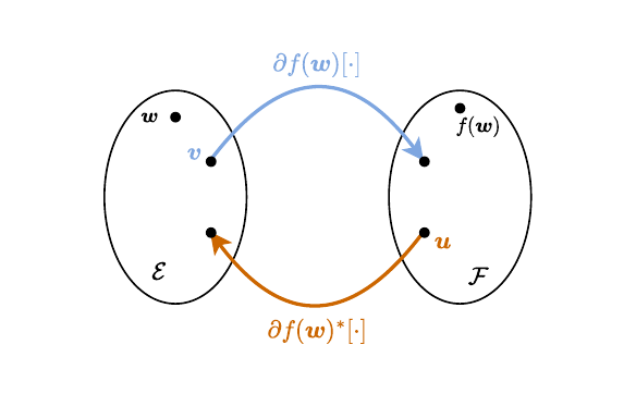
Figure 2.5: Jacobian-vector product (JVP) $\v \mapsto \partial f(\w)[\v]$ and vector-Jacobian product (VJP) $\u \mapsto \partial f(\w)^*[\u]$ , seen as linear maps.

2.3.6 Chain rule using linear maps

The chain rule presented before in terms of Jacobian matrices can readily be formulated to take advantage of the implementations of the JVP and VJP as linear maps.

Proposition 2.6 (Chain rule, general case)

Consider $f:\cE \rightarrow \cF$ and $g:\cF \rightarrow \cG$ , where $\cE$ , $\cF$ and $\cG$ are Euclidean spaces. If $f$ is differentiable at $\w \in \cE$ and $g$ is differentiable at $f(\w) \in \cF$ , then the composition $g \circ f$ is differentiable at $\w \in \cE$ . Its JVP is given for all $\v \in \cE$ by $\partial (g\circ f)(\w)[\v] = \partial g(f(\w))[\partial f(\w)[\v]]$ and its VJP is given for all $\u \in \cG$ by $\partial (g\circ f)(\w)^*[\u] = \partial f(\w)^*[\partial g(f(\w))^*[\u]].$

The proof follows the one of Proposition 2.2. This is illustrated in Fig. 2.6. When the last function is scalar-valued, which is often the case in machine learning, we obtain the following simplified result.

Proposition 2.7 (Chain rule, scalar case)

Consider $f:\cE \rightarrow \cF$ and $g: \cF \rightarrow \RR$ , the gradient of the composition is given by $\nabla (g\circ f)(\w) = \partial f(\w)^* [\nabla g(f(\w))].$

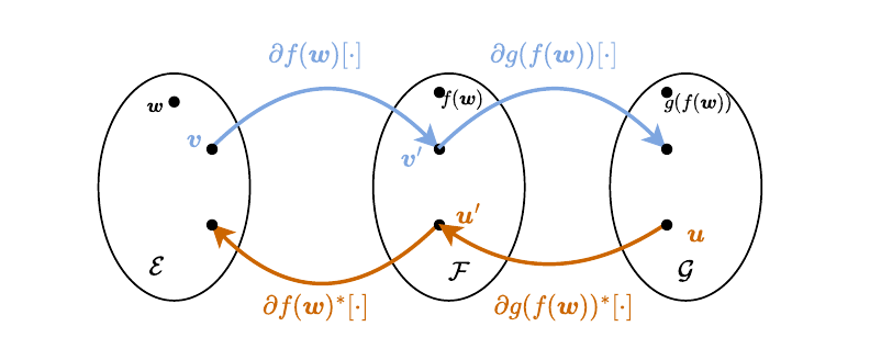
Figure 2.6: Chain rule using JVP and VJP linear maps.

2.3.7 Functions of multiple inputs (fan-in)

Oftentimes, the inputs of a function do not belong to only one Euclidean space but to a product of them. An example is $f(\x, \W) \coloneqq \W \x$ , which is defined on $\cE \coloneqq \RR^D \times \RR^{M \times D}$ . In such a case, it is convenient to generalize the notion of partial derivatives to handle blocks of inputs.

Consider a function $f(\w_1, \ldots, \w_S)$ defined on $\cE \coloneqq \cE_1 \times \ldots \times \cE_S$ , where $\w_i \in \cE_i$ . We denote the partial derivative with respect to the $i$ ^th input $\w_i$ along $\v_i \in \cE_i$ as $\partial_i f(\w_1, \ldots, \w_S)[\v_i]$ . Equipped with this notation, we can analyze how JVPs or VJPs are decomposed along several inputs.

Proposition 2.8 (Multiple inputs)

Consider a differentiable function of the form $f(\w) = f(\w_1, \dots, \w_S)$ with signature $f \colon \cE \to \cF$ , where $\w \coloneqq (\w_1, \dots, \w_S) \in \cE$ and $\cE \coloneqq \cE_1 \times \dots \times \cE_S$ . Then the JVP with the input direction $\v = (\v_1, \dots, \v_S) \in \cE$ is given by $\begin{align*} \partial f(\w)[\v] &= \partial f(\w_1, \dots, \w_S)[\v_1, \dots, \v_S] \in \cF \\ &= \sum_{i=1}^S \partial_i f(\w_1, \dots, \w_S)[\v_i]. \end{align*}$ The VJP with the output direction $\u \in \cF$ is given by $\begin{align*} \partial f(\w)^*[\u] &= \partial f(\w_1, \dots, \w_S)^*[\u] \in \cE \\ &= (\partial_1 f(\w_1, \dots, \w_S)^*[\u], \dots, \partial_S f(\w_1, \dots, \w_S)^*[\u]). \end{align*}$

Example 2.8 (Matrix-vector product)

Consider $f(\x, \W) \coloneqq \W \x$ , where $\W \in \RR^{M \times D}$ and $\x \in \RR^D$ . This corresponds to setting $\cE \coloneqq \cE_1 \times \cE_2 \coloneqq \RR^D \times \RR^{M \times D}$ and $\cF \coloneqq \RR^M$ . For the JVP, letting $\v \in \cE_1$ and $\V \in \cE_2$ , we obtain $\partial f(\x, \W)[\v, \V] = \W \v + \V \x \in \cF.$ We can also access the individual JVPs as $\begin{aligned} \partial_1 f(\x, \W)[\v] &= \W \v \in \cF, \\ \partial_2 f(\x, \W)[\V] &= \V \x \in \cF. \end{aligned}$ For the VJP, letting $\u \in \cF$ , we obtain $\partial f(\x, \W)^*[\u] = (\W^\top \u, \u \x^\top) \in \cE.$ We can access the individual VJPs by $\begin{aligned} \partial_1 f(\x, \W)^*[\u] &= \W^\top \u \in \cE_1, \\ \partial_2 f(\x, \W)^*[\u] &= \u \x^\top \in \cE_2. \end{aligned}$

Remark 2.5 (Nested inputs)

It is sometimes convenient to group inputs into meaningful parts. For instance, if the input is naturally broken down into two parts $\x = (\x_1, \x_2)$ , where $\x_1$ is a text part and $\x_2$ is an image part, and the network parameters are naturally grouped into three layers $\w = (\w_1, \w_2, \w_3)$ , we can write $f(\x, \w) = f((\x_1, \x_2), (\w_1, \w_2, \w_3))$ . This is mostly a convenience and we can again reduce it to a function of a single input, thanks to the linear map perspective in Euclidean spaces.

Remark 2.6 (Hiding away inputs)

It will often be convenient to ignore inputs when differentiating. We use the semicolon for this purpose. For instance, a function of the form $L(\w; \x, \y)$ (notice the semicolon) has signature $L \colon \cW \to \RR$ because we treat $\x$ and $\y$ as constants. Therefore, the gradient is $\nabla L(\w; \x, \y) \in \cW$ . On the other hand, the function $L(\w, \x, \y)$ (notice the comma) has signature $L \colon \cW \times \cX \times \cY \to \RR$ so its gradient is $\nabla L(\w, \x, \y) \in \cW \times \cX \times \cY$ . If we need to access partial gradients, we use indexing, e.g., $\nabla_1 L(\w, \x, \y) \in \cW$ or $\nabla_\w L(\w, \x, \y) \in \cW$ when there is no ambiguity.

2.3.8 Functions with multiple outputs (fan-out)

Similarly, it is often convenient to deal with functions that have multiple outputs.

Proposition 2.9 (Multiple outputs)

Consider a differentiable function of the form $f(\w) \coloneqq (f_1(\w), \dots, f_T(\w))$ , with signatures $f \colon \cE \to \cF$ and $f_i \colon \cE \to \cF_i$ , where $\cF \coloneqq \cF_1 \times \dots \times \cF_T$ . Then the JVP with the input direction $\v \in \cE$ is given by $\begin{align*} \partial f(\w)[\v] = (\partial f_1(\w)[\v], \dots, \partial f_T(\w)[\v]) \in \cF. \end{align*}$ The VJP with the output direction $\u = (\u_1, \dots, \u_T) \in \cF$ is $\begin{align*} \partial f(\w)^*[\u] &= \partial f(\w)^*[\u_1, \dots, \u_T] \in \cE \\ &= \sum_{i=1}^T \partial f_i(\w)^*[\u_i]. \end{align*}$

Combined with the chain rule, we obtain that the Jacobian of $h(\w) \coloneqq g(f(\w)) = g(f_1(\w), \dots, f_T(\w))$ is $\partial h(\w) = \sum_{i=1}^T \partial_i g(f(\w)) \circ \partial f_i(\w)$ and therefore the JVP is $\partial h(\w) [\v] = \sum_{i=1}^T \partial_i g(f(\w)) [\partial f_i(\w)[\v]].$

2.3.9 Extensions to non-Euclidean linear spaces

So far, we focused on Euclidean spaces, i.e., linear spaces with a finite basis. However, the notions studied earlier can be generalized to more generic spaces.

For example, directional derivatives (see Definition 2.12) can be defined in any linear space equipped with a norm and complete with respect to this norm. Such spaces are called Banach spaces. Completeness is a technical assumption that requires that any Cauchy sequence converges (a Cauchy sequence is a sequence whose elements become arbitrarily close to each other as the sequence progresses). A function $f: \cE \rightarrow \cF$ defined from a Banach space $\cE$ onto a Banach space $\cF$ is then called Gateaux differentiable if its directional derivative is defined along any direction (where limits are defined w.r.t. the norm in $\cF$ ). Some authors also require the directional derivative to be linear to define a Gateaux differentiable function.

Fréchet differentiability can also naturally be generalized to Banach spaces. The only difference is that, in generic Banach spaces, the linear map $l$ satisfying Definition 2.12 must be continuous, i.e., there must exist $C>0$ , such that $l[\v] \leq C \|\v\|$ , where $\|\cdot\|$ is the norm in the Banach space $\cE$ .

The definitions of gradient and VJPs require in addition a notion of inner product. They can be defined in Hilbert spaces, that is, linear spaces equipped with an inner product and complete with respect to the norm induced by the inner product (they could also be defined in a Banach space by considering operations in the dual space, see, e.g. (Clarke et al., 2008)). The existence of the gradient is ensured by Riesz’s representation theorem which states that any continuous linear form in a Hilbert space can be represented by the inner product with a vector. Since for a differentiable function $f: \cE \rightarrow \RR$ , the JVP $\partial f(\w): \cE \rightarrow \RR$ is a linear form, Riesz’s representation theorem ensures the existence of the gradient as the element $g \in \cE$ such that $\partial f(\w) \v = \langle g, \v\rangle$ for any $\v \in \cE$ . The VJP is also well-defined as the adjoint of the JVP w.r.t. the inner product of the Hilbert space.

As an example, the space of squared integrable functions on $\RR$ is a Hilbert space equipped with the inner product $\langle a, b \rangle \coloneqq \int a(x)b(x) dx.$ Here, we cannot find a finite number of functions that can express all possible functions on $\RR$ . Therefore, this space is not a mere Euclidean space. Nevertheless, we can consider functions on this Hilbert space (called functionals to distinguish them from the elements of the space). The associated directional derivatives and gradients, can be defined and are called respectively, functional derivative and functional gradient, see, e.g., Frigyik et al. (2008) and references therein.

2.4 Second-order differentiation

2.4.1 Second derivatives

For a single-input, single-output differentiable function $f:\RR \rightarrow \RR$ , its derivative at any point is itself a function $f': \RR \rightarrow \RR$ . We may then consider the derivative of the derivative at any point: the second derivative.

Definition 2.14 (Second derivative)

The second derivative $f^{(2)}(w)$ of a differentiable function $f: \RR \rightarrow \RR$ at $w \in \RR$ is defined as the derivative of $f'$ at $w$ , that is, $f^{(2)}(w) \coloneqq \lim_{\delta \rightarrow 0} \frac{f'(w+\delta) - f'(w)}{\delta},$ provided that the limit is well-defined. If the second derivative of a function $f$ is well-defined at $w$ , the function is said to be twice differentiable at $w$ . The second derivative is also denoted $f''$ .

If $f$ has a small second derivative at a given $w$ , the derivative around $w$ is almost constant. That is, the function behaves like a line around $w$ , as illustrated in Fig. 2.7. Hence, the second derivative is usually interpreted as the curvature of the function at a given point.

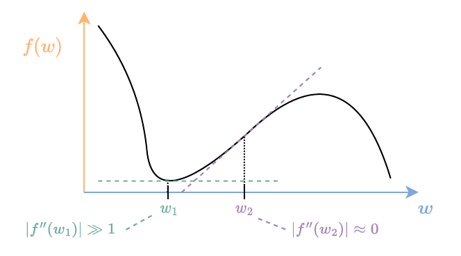
Figure 2.7: Points at which the second derivative is small are points along which the function is well approximated by its tangent line. On the other hand, points with large second derivative tend to be badly approximated by the tangent line.

2.4.2 Second directional derivatives

For a multi-input function $f:\RR^P \rightarrow \RR$ , we saw that the directional derivative encodes infinitesimal variations of $f$ along a given direction. To analyze the second derivative, the curvature of the function at a given point $\w$ , we can consider the variations along a pair of directions, as defined below.

Definition 2.15 (Second directional derivative)

The second directional derivative of $f:\RR^P \rightarrow \RR$ at $\w\in \RR^P$ along $\v, \v' \in \RR^P$ is defined as the directional derivative of $\w \mapsto \partial f(\w)[\v]$ along $\v'$ , that is, $\partial^2 f(\w)[\v, \v'] \coloneqq \lim_{\delta \rightarrow 0} \frac{\partial f(\w + \delta \v')[\v] - \partial f(\w)[\v]}{\delta},$ provided that $\partial f(\w)[\v]$ is well-defined around $\w$ and that the limit exists.

Of particular interest are the variations of a function around the canonical directions: the second partial derivatives, defined as $\partial_{i j}^2 f(\w) \coloneqq \partial^2 f(\w)[\e_i, \e_j]$ for $\e_i$ , $\e_j$ the $i$ ^th and $j$ ^th canonical directions in $\RR^P$ , respectively. In Leibniz notation, the second partial derivatives are denoted $\partial_{i j}^2 f(\w) = \frac{\partial^2 f(\w)}{\partial w_i \partial w_j}.$

2.4.3 Hessians

For a multi-input function, twice differentiability is simply defined as the differentiability of any directional derivative $\partial f(\w)[\v]$ w.r.t. $\w$ .

Definition 2.16 (Twice differentiability)

A function $f: \RR^P \rightarrow \RR$ is twice differentiable at $\w \in \RR^P$ if it is differentiable and $\partial f: \RR^P \rightarrow (\RR^P \rightarrow\RR)$ is also differentiable at $\w$ .

As a result, the second directional derivative is a bilinear form.

Definition 2.17 (Bilinear map, bilinear form)

A function $b: \RR^P \times \RR^P \rightarrow \RR^M$ is a bilinear map if $b[\v, \cdot]: \RR^P \rightarrow \RR$ is linear for any $\v$ and $b[\cdot, \v']$ is linear for any $\v'$ . That is, $b[\v, \v'] = \sum_{i=1}^P v_i b[\e_i, \v'] = \sum_{i=1}^{P} \sum_{j=1}^P v_iv_j' b[\e_i, \e_j],$ for $\v = \sum_{i=1}^P v_i \e_i$ and $\v' = \sum_{i=1}^P v_i' \e_i$ . A bilinear map with values in $\RR$ , $b: \RR^P \times \RR^P \rightarrow \RR$ , is called a bilinear form.

The second partial derivatives are gathered in the Hessian and the second directional derivatives can be computed from it.

Definition 2.18 (Hessian)

The Hessian of a twice differentiable function $f:\RR^P \rightarrow \RR$ at $\w$ is the $P \times P$ matrix gathering all second partial derivatives, $\nabla^2 f(\w) \coloneqq \begin{pmatrix} \partial_{11} f(\w) & \ldots & \partial_{1P} f(\w) \\ \vdots & \ddots & \vdots \\ \partial_{P1} f(\w) & \ldots & \partial_{PP} f(\w) \end{pmatrix} \in \RR^{P \times P},$ provided that all second partial derivatives are well-defined.

The second directional derivative at $\w$ is bilinear in any direction $\v = \sum_{i=1}^P v_i \e_i$ and $\v' = \sum_{i=1}^P v_i' \e_i$ . Therefore, $\partial^2 f(\w)[\v, \v'] = \sum_{i, j = 1}^{P} v_i v_j'\partial^2 f(\w)[\e_i, \e_j] = \langle \v, \nabla^2 f(\w) \v'\rangle.$

Given the gradient of $f$ , the Hessian is equivalent to the transpose of the Jacobian of the gradient. By slightly generalizing the notation $\nabla$ to denote the transpose of the Jacobian of a function (which matches its definition for single-output functions), we have that the Hessian can be expressed as $\nabla^2 f(\w) = \nabla (\nabla f)(\w)$ , which justifies its notation.

Similarly as for the differentiability of a function $f$ , twice differentiability of $f$ at $\w$ is equivalent to having the second partial derivatives not only defined but also continuous in a neighborhood of $\w$ . Remarkably, by requiring twice differentiability, i.e., continuous second partial derivatives, the Hessian is guaranteed to be symmetric (Schwarz, 1873).

Proposition 2.10 (Symmetry of the Hessian)

If a function $f:\RR^P \rightarrow \RR$ is twice differentiable at $\w$ , then its Hessian $\nabla^2 f(\w)$ is symmetric, that is, $\partial_{i j}^2 f(\w) = \partial_{j i}^2 f(\w)$ for any $i, j \in \{1, \ldots P\}$ .

The symmetry of the Hessian means that it can alternatively be written as $\nabla^2 f(\w) = (\partial_{ji}^2f(\w))_{i, j=1}^P = \jac (\nabla f)(\w)$ , i.e., the Jacobian of the gradient of $f$ .

2.4.4 Hessian-vector products

Similarly to the Jacobian, we can exploit the formal definition of the Hessian as a bilinear form to extend its definition to Euclidean spaces. In particular, we can define the notion of Hessian-vector product.

Definition 2.19 (Hessian-vector product)

If a function $f: \cE \rightarrow \R$ defined on a Euclidean space $\cE$ with inner product $\langle\cdot, \cdot\rangle$ , is twice differentiable at $\w \in \cE$ , then for any $\v \in \cE$ , there exists $\v \mapsto \nabla^2 f(\w)[\v]$ , called the Hessian-vector product (HVP) of $f$ at $\w$ along $\v$ , such that for any $\v' \in \cE$ , $\partial^2 f(\w)[\v, \v'] = \langle \v', \nabla^2 f(\w)[\v]\rangle.$ In particular for $\cE = \RR^P$ , the HVP is $\nabla^2 f(\w)[\v]= (\partial^2 f(\w)[\v, \e_i])_{i=1}^P$ .

From an autodiff point of view, the HVP can be implemented in four different ways, as explained in Section 9.1.

2.4.5 Second-order Jacobians

The previous definitions naturally extend to multi-output functions $f: \cE \rightarrow \cF$ , where $f \coloneqq (f_1, \dots, f_M)$ , $f_j \colon \cE \to \cF_j$ and $\cF \coloneqq \cF_1 \times \dots \times \cF_M$ . The second directional derivative is defined by gathering the second derivatives of each coordinate’s function. That is, for $\w, \v, \v' \in \cE$ , $\partial^2 f(\w)[\v, \v'] = (\partial^2 f_j(\w)[\v, \v'])_{j=1}^M \in \cF.$ The function $f$ is twice differentiable if and only if all its coordinates are twice differentiable. The second directional derivative is then a bilinear map. We can then compute second directional derivatives as $\partial^2 f(\w)[\v, \v'] = \sum_{i,j=1}^P v_i v_j' \partial^2 f(\w)[\e_i, \e_j] = (\langle \v, \nabla^2 f_j(\w) \v'\rangle)_{j=1}^M.$ When $\cE = \RR^P$ and $\cF_j = \RR$ , so that $\cF = \RR^M$ , the bilinear map can be materialized as a tensor $\partial^2 f(\w) = (\partial^2 f(\w)[\e_i, \e_j])_{i,j=1}^P \in \RR^{M \times P \times P},$ the “second-order Jacobian” of $f$ . However, similarly to the Hessian, it is usually more convenient to apply the bilinear map to prescribed vectors $\v$ and $\v'$ than to materialize the second partial derivatives as a tensor.

2.5 Higher-order differentiation

2.5.1 Higher-order derivatives

Derivatives can be extended to any order. Formally, the $n$ ^th derivative can be defined inductively as follows for a single-input, single-output function.

Definition 2.20 ( $n$ ^th order derivative)

The $n$ ^th derivative $f^{(n)}$ of a function $f:\RR \rightarrow \RR$ at $w \in \RR$ is defined as $f^{(n)}(w) \coloneqq (f^{(n-1)})'(w) = \lim_{\delta \rightarrow 0} \frac{f^{(n-1)}(w+\delta) - f^{(n-1)}(w)}{\delta}$ provided that $f^{(n-1)}$ is differentiable around $w$ and that the limit exists. In such a case, the function is said to be $n$ times differentiable at $w$ .

2.5.2 Higher-order directional derivatives

For a multi-input function $f$ , we can naturally extend the notion of directional derivative as follows.

Definition 2.21 ( $n$ ^th order directional derivative)

The $n$ ^th directional derivative of $f: \RR^P \rightarrow \R$ at $\w \in \RR^P$ along $\v_1, \ldots, \v_n$ is defined as $\begin{align*} & \partial^n f(\w)[\v_1, \ldots, \v_n] \\ & = \partial (\partial^{n-1}f(\w)[\v_1, \ldots, \v_{n-1}])[\v_n] \\ & = \lim_{\delta \rightarrow 0} \frac{ \partial f(\w + \delta \v_n)[\v_1, \ldots, \v_{n-1}] - \partial f(\w)[\v_1, \ldots, \v_{n-1}] }{ \delta } \end{align*}$

A multi-input function $f$ is $n$ -times differentiable if it is $n-1$ differentiable and its $n-1$ directional derivative along any direction is differentiable. As a consequence the $n$ ^th directional derivative is a multilinear form.

Definition 2.22 (Multilinear map, multilinear form)

A function $c: \otimes_{i=1}^n \RR^P \rightarrow \RR^M$ is a multilinear map if it is linear in each coordinate given all others fixed, that is, if $\v_j \mapsto c[\v_1,\ldots,\v_j,\ldots, \v_n]$ is linear in $\v_j$ for any $j \in [n]$ . It is a multilinear form if it has values in $\RR$ .

The $n$ ^th order directional derivative is then given by $\partial^n f(\w)[\v_1, \ldots, \v_n] = \sum_{i_1, \ldots, i_n=1}^P v_{1,i_1} \ldots v_{n, i_n} \partial^n f(\w)[\e_{i_1}, \ldots, \e_{i_n}].$ The $n$ ^th order partial derivatives can be materialized as an $n$ ^th order tensor $\nabla^n f(\w) = (\partial^n f(\w)[\e_{i_1}, \ldots, \e_{i_n}])_{i_1, \ldots, i_n=1}^P \in \RR^{P \times \ldots \times P}.$

2.5.3 Higher-order Jacobians

All above definitions extend directly to the case of multi-output functions $f:\cE \rightarrow \cF$ , where $\cF \coloneqq \cF_1 \times \dots \times \cF_M$ . The $n$ ^th directional derivatives are then $\partial^n f(\w)[\v_1, \ldots, \v_n] = (\partial^n f_j(\w)[\v_1, \ldots, \v_n])_{j=1}^M.$ The function $f$ is then $n$ times differentiable if it is $n-1$ differentiable and its $n-1$ directional derivative along any direction is differentiable. As a consequence, the $n$ ^th directional derivative is a multilinear map. The $n$ ^th directional derivative can be decomposed into partial derivatives as $\partial^n f(\w)[\v_1, \ldots, \v_n] = \sum_{i_1, \ldots, i_n=1}^P v_{1,i_1} \ldots v_{n, i_n} \partial^n f(\w)[\e_{i_1}, \ldots, \e_{i_n}].$ When $\cE = \RR^P$ and $\cF = \RR^M$ , the $n$ ^th order partial derivatives can be materialized by an $(n+1)$ ^th order tensor $\partial^n f(\w) = (\partial^n f_j(\w)[\e_{i_1}, \ldots, \e_{i_n}])_{j=1, i_1, \ldots, i_n=1}^{M, P, \ldots, P} \in \RR^{M \times P \times \ldots \times P}.$

2.5.4 Taylor expansions

With Landau’s little $o$ notation, we have seen that if a function is differentiable, it is approximated by a linear function in $\v$ , $f(\w+\v) = f(\w) + \langle \nabla f(\w), \v\rangle + o(\|\v\|_2).$ Such an expansion of the function up to its first derivative is called the first-order Taylor expansion of $f$ around $\w$ .

If the function $f$ is twice differentiable, we can approximate it by a quadratic in $\v$ , leading to the second-order Taylor expansion of $f$ around $\w$ , $f(\w+\v) = f(\w) + \langle \nabla f(\w), \v \rangle + \frac{1}{2}\langle \v, \nabla^2 f(\w) \v\rangle + o(\|\v\|_2^2).$ Compared to the first-order Taylor approximation, it is naturally more accurate around $\w$ , as reflected by the fact that $\|\v\|_2^3 \leq \|\v\|_2^2$ for $\|\v\|_2 \le 1$ .

More generally, we can build the $\n$ ^th order Taylor expansion of a $n$ times differentiable function $f \colon \RR^P \to \RR^M$ around $\w \in \RR^P$ by $\begin{align*} f(\w+\v) & = f(\w) + \partial f(\w)[\v] + \frac{1}{2} \partial^2 f(\w)[\v, \v] + \ldots \\ & + \frac{1}{n!} \partial^n f(\w)[\underbrace{\v, \ldots, \v}_{n \, \mathrm{times}}] + o(\|\v\|_2^{n}). \end{align*}$ Note that, using the change of variable $\w' = \w + \v \iff \v = \w' - \w$ , it is often convenient to write the $n$ ^th Taylor expansion of $f(\w')$ around $\w$ as $f(\w') = f(\w) + \sum_{j=1}^{n} \frac{1}{j!} \partial^j f(\w)[\underbrace{\w' - \w, \ldots, \w' - \w}_{j \, \mathrm{times}}] + o(\|\w' - \w\|_2^{n}).$ Taylor expansions will prove useful in Chapter 7 for computing derivatives by finite differences.

2.6 Differential geometry

In this chapter, we progressively generalized the notion of derivative from real numbers to vectors and variables living in a linear space (a.k.a. vector space), either finite dimensional or infinite dimensional. We can further generalize these notions by considering a local notion of linearity. This is formalized by smooth manifolds in differential geometry, whose terminology is commonly adopted in the automatic differentiation literature and software. In this section, we give a brief overview of derivatives on smooth manifolds (simply referred to as manifolds), and refer to Boumal (2023) for a complete introduction.

2.6.1 Differentiability on manifolds

Essentially, a manifold is a set that can be locally approximated by a Euclidean space. The most common example is a sphere like the Earth. Seen from the Moon, the Earth is not a plane, but locally, at a human level, it can be seen as a flat surface. Euclidean spaces are also trivial examples of manifolds. A formal characterization of the sphere as a manifold is presented in Example 2.9. For now, we may think of a “manifold” as some set (e.g., the sphere) contained in some ambient Euclidean space; note however that manifolds can be defined generally without being contained in a Euclidean space (Boumal, 2023, 8). Differentiability in manifolds is simply inherited from the notion of differentiability in the ambient Euclidean space.

Definition 2.23 (Differentiability of restricted functions)

Let $\cM$ and $\cN$ be manifolds. A function $f: \mathcal{M} \rightarrow \mathcal{N}$ defined from $\mathcal{M} \subseteq \cE$ to $\mathcal{N} \subseteq \cF$ , with $\cE$ and $\cF$ Euclidean spaces, is differentiable if $f$ is the restriction of a differentiable function $\bar f:\cE \rightarrow \cF$ , so that $f$ coincides with $\bar f$ on $\mathcal{M}$ .

Our objective is to formalize the directional derivatives and gradients for functions defined on manifolds. This formalization leads to the definitions of tangent spaces and cotangent spaces, and the associated generalizations of JVP and VJP operators as pushforward and pullback operators, respectively.

2.6.2 Tangent spaces and pushforward operators

To generalize the notion of directional derivatives of a function $f$ , the one property we want to preserve is the chain rule. Rather than starting from the variations of $f$ at a given point along a direction, we start with the variations of $f$ along curves. Namely, on a manifold like the sphere $\cS^P$ in $\RR^P$ , we can look at curves $\alpha: \R \rightarrow \cS^P$ passing through $\w \in \cS^P$ at time $0$ , that is, $\alpha(0) = \w$ . For single-input functions like $\alpha$ , we denote for simplicity $\alpha'(0) \coloneqq (\alpha_1'(0), \ldots, \alpha_P'(0))$ . The directional derivative of a function $f$ must typically serve to define the derivative of $f\circ \alpha$ at $0$ , such that $(f\circ \alpha)'(0) = \partial f(\w)[\alpha'(0)]$ . In the case of the sphere, as illustrated in Fig. 2.8, the derivative $\alpha'(0)$ of a curve $\alpha$ passing through a point $\w$ is always tangent to the sphere at $\w$ . The tangent plane to the sphere at $\w$ then captures all possible relevant vectors to pass to the JVP we are building. To define the directional derivative of a function $f$ on a manifold, we therefore restrict ourselves to an operator defined on the tangent space $\cT_\w\cM$ , whose definition below is simplified for our purposes.

Definition 2.24 (Tangent space)

The tangent space of a manifold $\cM$ at $\w \in \cM$ is defined as $\cT_\w \mathcal{M} \coloneqq \{\v = \alpha'(0) \ \mbox{for any} \ \alpha: \RR \rightarrow \cM \ \mbox{differentiable s.t.} \ \alpha(0) = \w \}.$

In the case of the sphere in Fig. 2.8, the tangent space is a plane, that is, a Euclidean space. This property is generally true: tangent spaces are Euclidean spaces, enabling us to define directional derivatives as linear maps. Now, if $f$ is differentiable and goes from a manifold $\cM$ to a manifold $\cN$ , then $f\circ \alpha$ is a differentiable curve in $\cN$ . Therefore, $(f\circ \alpha)'(0)$ is the derivative of a curve passing through $f(\w)$ at $0$ and is tangent to $\cN$ at $f(\w)$ . Hence, the directional derivative of $f: \cM \rightarrow \cN$ at $\w$ can be defined as a function from the tangent space $\cT_\w \mathcal{M}$ of $\cM$ at $\w$ onto the tangent space $\cT_{f(\w)} \mathcal{N}$ of $\cN$ at $f(\w)$ . Overall, we built the directional derivative (JVP) by considering how a composition of $f$ with any curve $\alpha$ pushes forward the derivative of $\alpha$ into the derivative of $f\circ \alpha$ . The resulting JVP is called a pushforward operator in differentiable geometry.

Definition 2.25 (Pushforward operator)

Given two manifolds $\cM$ and $\cN$ , the pushforward operator of a differentiable function $f: \mathcal{M} \rightarrow \mathcal{N}$ at $\w \in \mathcal{M}$ is the linear map $\partial f(\w): \mathcal{T}_\w \mathcal{M} \rightarrow \mathcal{T}_{f(\w)} \mathcal{N}$ defined by $\partial f(\w)[\v] \coloneqq (f\circ \alpha)'(0),$ for any $\v \in \cT_\w \cM$ such that $\v = \alpha'(0)$ , where $\alpha: \RR \rightarrow \cM$ is a differentiable curve passing through $\w$ at $0$ , i.e., $\alpha(0) = \w$ .

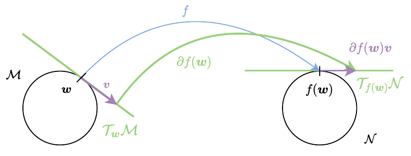
Figure 2.8: A differentiable function $f$ defined from a sphere $\cM$ to a sphere $\cN$ defines a push-forward operator that maps tangent vectors (derivatives of functions on the sphere passing through $\w$ ) in the tangent space $\cT_{\w} \cM$ to tangent vectors of $\cN$ at $f(\w)$ in the tangent space $\cT_{f(\w)}\cN$ .

2.6.3 Cotangent spaces and pullback operators

To generalize the JVP, we composed $f: \cM \rightarrow \cN$ with any single-input function $\alpha: \RR\rightarrow \cM$ giving values on the manifold. The derivative of any such $\alpha$ is then pushed forward from $\cT_\w \mathcal{M}$ to $\cT_{f(\w)} \mathcal{N}$ by the action of $f$ . To define the VJP, we take a symmetric approach. We consider all single-output differentiable functions $\beta: \cN \rightarrow \RR$ defined on $\y \in \cN$ with $\y=f(\w)$ for some $\w \in \cM$ . We then want to pull back the derivatives of $\beta$ when precomposing it by $f$ . Therefore, the space on which the VJP acts is the space of directional derivatives of any $\beta: \cN \rightarrow \RR$ at $\y$ , defining the cotangent space.

Definition 2.26 (Cotangent space)

The cotangent space of a manifold $\cN$ at $\y \in \cN$ is defined as $\begin{align*} \cT_\y^* \mathcal{N} & = \{ u = \partial \beta(\y) \ \mbox{for any} \ \beta: \cN \rightarrow \RR \ \mbox{differentiable} \} \\ & = \{u: \cT_\y \mathcal{N} \rightarrow \RR \ \mbox{for any linear map} \ u \}, \end{align*}$

Note that elements of the cotangent space are linear mappings, not vectors. This distinction is important to define the pullback operator as an operator on functions as done in measure theory. From a linear algebra viewpoint, the cotangent space is exactly the dual space of $\cT_\y\mathcal{N}$ , that is, the set of linear maps from $\cT_\y \mathcal{N}$ to $\RR$ , called linear forms. As $\cT_\y \mathcal{N}$ is a Euclidean space, its dual space $\cT_\y^* \mathcal{N}$ is also a Euclidean space. The pullback operator is then defined as the operator that gives access to directional derivatives of $\beta \circ f$ given the directional derivative of $\beta$ at $f(\w)$ .

Definition 2.27 (Pullback operator)

Given two manifolds $\cM$ and $\cN$ , the pullback operator of a differentiable function $f: \mathcal{M} \rightarrow \mathcal{N}$ at $\w \in \mathcal{M}$ is the linear map $\partial f(\w)^\star: \mathcal{T}_{f(\w)}^*\mathcal{N} \rightarrow \mathcal{T}_{\w}^* \mathcal{M}$ defined by $\partial f(\w)^\star u \coloneqq \partial (\beta \circ f)(\w),$ for any $u \in \cT_{f(\w)} \mathcal{N}^*$ such that $\partial \beta( f(\w)) = u$ , for a differentiable function $\beta: \cN \rightarrow \RR$ .

Contrary to the pushforward operator that acts on vectors, the pullback operator acts on linear forms. Hence, the slight difference in notation between $\partial f(\w)^\star$ and $\partial f(\w)^*$ , the adjoint operator of $\partial f(\w)$ . To properly define the adjoint operator $\partial f(\w)^*$ , we need a notion of inner product. Since tangent spaces are Euclidean spaces, we can define an inner product $\langle \cdot, \cdot \rangle_\w$ for each $\cT_\w \cM$ and $\w\in \cM$ , making $\cM$ a Riemannian manifold. Equipped with these inner products, the cotangent space can be identified with the tangent space, and we can define gradients.

Definition 2.28 (Gradients in Riemannian manifolds)

Let $\cM$ be a Riemannian manifold equipped with inner products $\langle \cdot, \cdot\rangle_\w$ . For any cotangent vector $u \in \cT_\w^* \mathcal{M}$ , with $\w \in \cM$ , there exists a unique tangent vector $\u \in \cT_\w \mathcal{M}$ such that $\forall \v \in \cT_\w \mathcal{M}, \ u[\v] = \langle \u, \v\rangle_\w.$ In particular for any differentiable function $f: \cM \rightarrow \RR$ , we can define the gradient of $f$ as the unique tangent vector $\nabla f(\w) \in \cT_\w \mathcal{M}$ such that $\forall \v \in \cT_\w \mathcal{M}, \ \partial f(\w)[\v] = \langle \nabla f(\w), \v\rangle.$

Therefore, rather than pulling back directional derivatives, we can pull back gradients. The corresponding operator is then naturally the adjoint $\partial f(\w)^*$ of the pushforward operator. Namely, given two Riemannian manifolds $\cM$ and $\cN$ , and a differentiable function $f: \mathcal{M} \rightarrow \mathcal{N}$ , we have $\left(\partial f(\w)^\star u\right)[\v] = \langle \partial f(\w)^*[\u], \v\rangle \ \mbox{for any} \ \v \in \cT_\w \mathcal{M}$ for $u = \langle \cdot, \u\rangle \in \cT_{f(\w)}^* \mathcal{N}$ represented by $\u \in \cT_{f(\w)} \mathcal{N}$ .

Function	$f$	$\cM \rightarrow \cN$
Push-forward	$\partial f(\w)$	$\cT_\w\mathcal{M} \rightarrow \cT_{f(\w)} \mathcal{N}$
Pullback	$\partial f(\w)^\star$	$\cT_{f(\w)}^\mathcal{N} \rightarrow \cT_\w^ \mathcal{M}$
Adjoint of pushforward	$\partial f(\w)^*$	$\cT_{f(\w)} \mathcal{N} \rightarrow \cT_\w \mathcal{M}$

Table 2.1: For a differentiable function $f$ defined from a manifold $\cM$ onto a manifold $\cN$ , the JVP is generalized with the notion of pushforward $\partial f(\w)$ . The counterpart of the pushforward is the pullback operation $\partial f(\w)^\star$ that acts on linear forms in the tangent spaces. For Riemannian manifolds, the pullback operation can be identified with the adjoint operator $\partial f(\w)^*$ of the pushforward operator as any linear form is represented by a vector.

Example 2.9 (The sphere as a manifold)

The sphere $\cS^P$ in $\RR^P$ is defined as the set of points $\w\in \RR^P$ , satisfying $c(\w) \coloneqq \langle \w, \w \rangle - 1 = 0$ , with JVP $\partial c(\w)[\v] = 2\langle \w, \v\rangle$ .

Let us first understand why we may locally see the sphere $\cS^P$ as a space of dimension $P-1$ . Take the hemisphere $\cH = \{\w \in \cS^P: w_P \geq 0\}$ , it can be entirely described by using the first $P-1$ coordinates of each point, the last one is simply given by $w_P= \sqrt{1- \sum_{i=1}^{P-1}w_i^2}$ . Formally, for any vector $\v = (v_1, \ldots, v_{P-1})$ of $P-1$ coordinates such that $\sum_{i=1}^{P-1} v_i^2 \leq 1$ , we can define $\psi_1(\v) \coloneqq \sqrt{1- \sum_{i=1}^{P-1} v_i^2}$ and $\psiv(\v) \coloneqq (v_1, \ldots, v_{P-1}, \psi_1(\v))$ . We have then $\langle \psiv(\v), \psiv(\v)\rangle = 1$ , that is $c(\psiv(\v)) = 0$ . We can then describe the hemisphere $\cH$ as the image of the unit ball $B = \{\v = (v_1, \ldots, v_{P-1}): \sum_{i=1}^{P-1} v_i^2 \leq 1\}$ in dimension $P-1$ through the mapping $\psi$ , that is, $\cH = \psi(B)$ . In particular, any open set on the hemisphere can be described as the mapping of an open set in $\RR^{P-1}$ . The reasoning applies to all hemispheres with different mappings, hence the local aspect of this viewpoint.

The tangent space can be naturally characterized in terms of the constraining function $c$ . Namely, the curve $\alpha: \RR \rightarrow \cS^P$ such that $\alpha(0) =\w$ satisfies for any $\delta\in \RR$ , $c(\alpha(\delta)) = \zeros$ . Hence, differentiating the implicit equation, we have $(c\circ \alpha)'(0) = \partial c(\w)[\alpha'(0)].$ That is, $\alpha'(0)$ is in the null space of $\partial c(\w)$ , denoted $\mathrm{Null}(\partial c(\w)) \coloneqq \{\v \in \RR^P: \partial c(\w)[\v] =0\}.$ The tangent space of $\cS^P$ at $\w$ is then $\begin{align*} \cT_\w \mathcal{M} & = \mathrm{Null}(2 \langle \w, \cdot\rangle) \\ & = \{ \v \in \RR^P: \langle \w, \v\rangle = 0\} \end{align*}$ We naturally recover that the tangent space is a Euclidean space of dimension $P-1$ , defined as the set of points orthogonal to $\w$ .

2.7 Generalized derivatives

While we largely focus on differentiable functions in this book, it is important to characterize non-differentiable functions. We distinguish here two cases: continuous functions and non-continuous functions. For the former case, there exist generalizations of the notion of directional derivative, gradient and Jacobian, presented below. For non-continuous functions, even if derivatives exist almost everywhere, they may be uninformative. For example, piecewise-constant functions, encountered in e.g. control flows (Chapter 5), are almost everywhere differentiable but with zero derivatives. In such cases, surrogate functions can be defined to ensure the differentiability of a program (Part IV).

2.7.1 Rademacher’s theorem

We first recall the definition of (locally) Lipschitz continuous function.

Definition 2.29 ((Locally) Lipschitz continuous function)

A function $f: \cE \rightarrow \cF$ , is Lipschitz continuous if there exists $C\geq 0$ such that for any $\x, \y \in \cE$ , $\|f(\x)- f(\y)\| \leq C\|\x-\y\|.$ A function $f: \cE \rightarrow \cF$ is locally Lipschitz continuous if for any $\x \in \cE$ , there exists a neighborhood $\cU$ of $\x$ such that $f$ restricted to $\cU$ is Lipschitz continuous.

Rademacher’s theorem (Rademacher, 1919) then ensures that $f$ is differentiable almost everywhere.

Proposition 2.11 (Rademacher’s theorem)

Let $\cE$ and $\cF$ denote Euclidean spaces. If $f: \cE \rightarrow \cF$ is locally Lipschitz-continuous, then $f$ is almost everywhere differentiable, that is, the set of points in $\cE$ at which $f$ is not differentiable is of (Lebesgue) measure zero.

See also Morrey Jr (2009) for a standard proof.

2.7.2 Clarke derivatives

Rademacher’s theorem hints that the definitions of directional derivatives, gradients and Jacobians may be generalized to locally Lipschitz continuous functions. This is what Clarke (1975) did in his seminal work, which laid the foundation of nonsmooth analysis. The first building block is a notion of generalized directional derivative.

Definition 2.30 (Clarke generalized directional derivative)

The Clarke generalized directional derivative of a locally Lipschitz continuous function $f: \cE \rightarrow \RR$ at $\w \in \cE$ in the direction $\v \in \cE$ is $\partial_C f(\w)[\v] \coloneqq \limsup_{\substack{\u \rightarrow \w \\ \delta \searrow 0}} \frac{f(\u + \delta \v) - f(\u)}{\delta},$ provided that the limit exists, where $\delta \searrow 0$ means that $\delta$ approaches $0$ by non-negative values, and where the limit superior is defined as $\limsup_{\x \rightarrow \a} f(\x) \coloneqq \lim_{\varepsilon \rightarrow 0} \sup\{f(\x) : \x \in B(\a, \varepsilon)\setminus\{\a\}\}$ for $B(\a, \varepsilon) \coloneqq \{\x \in \cE: \|\x-\a\|\leq \varepsilon \}$ the ball centered at $\a$ of radius $\varepsilon$ .

There are two differences with the usual definition of a directional derivative: (i) we consider slopes of the function in a neighborhood of the point rather than at the given point, (ii) we take a limit superior rather than a usual limit. The first point is rather natural in the light of Rademacher’s theorem: we can properly characterize variations on points where the function is differentiable, therefore we may take the limits of these slopes as a candidate slope for the point of interest. The second point is more technical but essential: it allows us to characterize the directional derivative as the supremum of some linear forms (Clarke et al., 2008). These linear forms in turn define a set of generalized gradients (Clarke et al., 2008, 2).

Definition 2.31 (Clarke generalized gradient)

A Clarke generalized gradient of a locally Lipschitz function $f: \cE\rightarrow \RR$ at $\w \in \cE$ is a point $\g \in \cE$ such that $\forall \v \in \cE$ $\partial_C f(\w)[\v] \geq \langle \g, \v \rangle.$ The set of Clarke generalized gradients is called the Clarke subdifferential of $f$ at $\w$ .

Definition 2.30 and Definition 2.31 can be used in non-Euclidean spaces, such as Banach or Hilbert spaces (Clarke et al., 2008). In Euclidean spaces, the Clarke generalized gradients can be characterized more simply thanks to Rademacher’s theorem (Clarke et al., 2008, Theorem 8.1). Namely, as shown below, they can be defined as a convex combination of limits of gradients of $f$ evaluated at a sequence in $\cE\setminus \Omega$ that converges to $\w$ .

Proposition 2.12 (Characterization of Clarke generalized gradients)

Let $f: \cE\rightarrow \RR$ be a locally Lipschitz continuous and denote $\Omega$ the set of points at which $f$ is not differentiable (Proposition 2.11). An element $\g \in \cE$ is a Clarke generalized gradient of $f$ at $\w \in \cE$ if and only if $\begin{align*} \g & \in \conv\left(\left\{ \lim_{n \rightarrow +\infty} \nabla f(\v_n) \colon (\v_n)_{n=1}^{+\infty} \ \mbox{s.t.} \ \v_n \in \cE\setminus \Omega, \ \v_n \underset{n \rightarrow + \infty}{\rightarrow} \w \right\}\right). \end{align*}$

In the above, the convex hull of a set $S\subseteq \cE$ , the set of convex combinations of elements of $S$ , is denoted $\conv(S) \coloneqq \{\lambda_1 \s_1 + \ldots + \lambda_m \s_m \ \colon m \in \NN, \ \lambda_i \geq 0, \sum_{i=1}^{m} \lambda_i = 1, \s_i \in S\}.$

The Jacobian of a function $f: \cE \rightarrow \cF$ between two Euclidean spaces can be generalized similarly (Clarke et al., 2008, Section 3.3).

Definition 2.32 (Clarke generalized Jacobian)

Let $f: \cE\rightarrow \cF$ be locally Lipschitz continuous and denote $\Omega$ the set of points at which $f$ is not differentiable (Proposition 2.11). A Clarke generalized Jacobian of $f$ at $\w \in \cE$ is an element $\mathbf{J}$ of $\conv\left(\left\{ \lim_{n \rightarrow +\infty} \jac f(\v_n) \colon (\v_n)_{n=1}^{+\infty} \ \mbox{s.t.} \ \v_n \in \cE\setminus \Omega, \ \v_n \underset{n \rightarrow + \infty}{\rightarrow} \w \right\}\right).$

For a continuously differentiable function $f: \cE \rightarrow \cF$ or $f:\cE \rightarrow \RR$ , there is a unique generalized gradient, recovering the usual gradient (Clarke et al., 2008, Proposition 3.1, page 78). The chain rule can be generalized to these objects (Clarke et al., 2008). Recently, (Bolte et al., 2022; Bolte and Pauwels; 2020) further generalized Clarke gradients through the definition of conservative gradients to define automatic differentiation schemes for nonsmooth functions.

2.8 Summary

The usual definition of derivatives of real-valued univariate functions extends to multivariate functions $f \colon \RR^P \to \RR$ through the notion of directional derivative $\partial f(\w)[\v]$ at $\w \in \RR^P$ in the direction $\v \in \RR^P$ .
To take advantage of the representation of $\w = \sum_{j=1}^P w_j \e_j$ using the canonical bases $\{\e_1, \dots, \e_P\}$ , the definition of differentiable functions requires the linearity of the directional derivative w.r.t. the direction $\v$ .
This requirement gives rise to the notion of gradient $\nabla f(\w) \in \RR^P$ , the vector that gathers the partial derivatives and further defines the steepest ascent direction at $\w$ .
For vector-input vector-output functions $f \colon \RR^P \to \RR^M$ , the directional derivative leads to the definition of Jacobian matrix $\jac f(\w) \in \RR^{M \times P}$ , the matrix which gathers all partial derivatives (notice that we use bold $\jac$ ). The chain rule is then the product of Jacobian matrices.
These notions can be extended to general Euclidean spaces, such as the spaces of matrices or tensors. For functions of the form $f \colon \cE \to \R$ , the gradient is $\nabla f(\w) \in \cE$ . More generally, for functions of the form $f \colon \cE \to \cF$ , the Jacobian $\partial f(\w)$ can be seen as a linear map (notice the non-bold $\partial$ ). The directional derivative at $\w \in \cE$ naturally defines a linear map $l[\vv] = \partial f(\w)[\vv]$ , where $\partial f(\w) \colon \cE \to \cF$ is called the Jacobian vector product (JVP) and captures the infinitesimal variation at $\w \in \cE$ along the input direction $\v \in \cE$ .
Its adjoint $\partial f(\w)^* \colon \cF \to \cE$ defines another linear map $l[\uv] = \partial f(\w)^*[\uv]$ called the vector Jacobian product (VJP) and captures the infinitesimal variation at $\w \in \cE$ along the output direction $\u \in \cF$ . The chain rule is then the composition of these linear maps.
For the particular case when we compose a scalar-valued function $\ell$ (such as a loss function) with a vector-valued function $f$ (such as a network function), the gradient is given by $\nabla (\ell \circ f)(\w) = \partial f(\w)^* \nabla \ell(f(\w))$ . This is why being able to apply the adjoint to a gradient, which as we shall see can be done with reverse-mode autodiff, is so pervasive in machine learning.
The definitions of JVP and VJP operators can further be generalized in the context of differentiable geometry. In that framework, the JVP amounts to the pushforward operator that acts on tangent vectors. The VJP amounts to the pullback operator that acts on cotangent vectors.
We also saw that the Hessian matrix of a function $f(\w)$ from $\RR^P$ to $\RR$ is denoted $\nabla^2 f(\w) \in \RR^{P \times P}$ . It is symmetric if the second partial derivatives are continuous. Seen as linear map, the Hessian leads to the notion of Hessian-vector product (HVP), which we saw can be reduced to the JVP or the VJP of $\nabla f(\w)$ .
The main take-away message of this chapter is that computing the directional derivative or the gradient of compositions of functions does not require computing intermediate Jacobians but only to evaluate linear maps (JVPs or VJPs) associated with these intermediate functions. The goal of automatic differentiation, presented in Chapter 8, is precisely to provide an efficient implementation of these maps for computation chains or more generally for computation graphs.