Part V Optimizing differentiable programs

Chapter 15Optimization basics

15.1 Objective functions

Consider a function $L$ , for example evaluating the error or “loss” $L(\w)$ achieved by a model with parameters $\w \in \cW$ , where $\cW=\RR^P$ . To find the best possible model parameterization, we seek to minimize $L(\w)$ , that is, to compute approximately $L^\star \coloneqq \inf_{\w \in \cW} L(\w),$ assuming that the infimum exists (i.e., $L(\w)$ is lower bounded). We will denote a solution, if it exists, by $\w^\star \in \argmin_{\w \in \cW} L(\w) \coloneqq \left\{\w \in \cW: L(\w) = \min_{\w' \in \cW} L(\w')\right\}.$ In general, an analytical solution is not available and computing such a minimum approximately requires an optimization algorithm. An optimization algorithm is an iterative procedure, which, starting from an initial point $\w \pow 0$ , outputs after $t$ iterations a point $\w \pow t$ that approximates the minimum of $L$ up to some accuracy $\varepsilon$ , i.e., $L(\w \pow t) - L^\star \leq \varepsilon. \tag{15.1}$

15.2 Oracles

To produce iterates $\w \pow 1, \w \pow 2, \dots$ that converge to a minimum, the algorithm naturally needs to have access to information about $L$ . For example, the algorithm needs a priori to be able to evaluate $L$ to know if it decreased its value or not. Such information about the function is formalized by the notion of oracles (Nemirovski and Yudin, 1983). Formally, oracles are procedures that an algorithm can call to access information about the objective $L(\w)$ at any given point $\w \in \cW$ . We usually mainly consider the following three oracles.

Zero-order oracle: evaluating the function $L(\w) \in \RR$ .
First-order oracle: evaluating the gradient $\nabla L(\w) \in \cW$ for $L$ differentiable.
Second-order oracle: evaluating the Hessian matrix $\nabla^2 L(\w)$ , or evaluating the Hessian-vector product (HVP) $\nabla^2 L(\w) \v \in \cW$ , for $L$ twice differentiable and any vector $\v \in \cW$ .

Given an oracle $\mathcal{O}$ for a function $L$ , we can formally define an optimization algorithm as a procedure which computes the next iterate as a function of all past and current information. Formally, an algorithm $\mathcal{A}$ builds a sequence $\w \pow 1, \ldots, \w \pow t$ from a starting point $\w \pow 0$ as $\w \pow {t+1} \coloneqq \mathcal{A}(\w \pow 0, \ldots, \w \pow t, \mathcal{O}(\w \pow 0), \ldots, \mathcal{O}(\w \pow t), \lambdav),$ where $\lambdav \in \Lambda \subseteq \RR^Q$ encapsulates some hyperparameters of the algorithm, such as the stepsize. Oftentimes, algorithms build the next iterate simply from the information collected at the current iterate, without using all past iterates. That is, they take the form $\w \pow {t+1} = \mathcal{A}(\w \pow t, \mathcal{O}(\w \pow t), \lambdav)$ . A classical example is the gradient descent algorithm, which uses a first-order oracle to compute iterates of the form $\w \pow {t+1} \coloneqq \w \pow t - \gamma \nabla L(\w \pow t),$ where the stepsize $\gamma$ is a hyperparameter of the algorithm. The notion of oracle therefore delineates different classes of algorithms. For instance, we may consider zero-order algorithms or first-order algorithms.

15.3 Variational perspective of optimization algorithms

One of the most basic optimization algorithms is the proximal point method, which produces $\w \pow {t+1}$ from $\w \pow t$ by $\w \pow {t+1} \coloneqq \argmin_{\w \in \cW} L(\w) + \frac{1}{2\gamma} \|\w - \w \pow t\|_2^2.$ In words, the next iterate is produced by solving a trade-off between minimizing the function $L$ and staying close to $\w^t$ . Unfortunately, the optimization problem involved in performing this parameter update is as difficult as the original optimization problem, making the proximal point method impractical.

As we shall see in Chapter 16 and Chapter 17, many optimization algorithms can be seen as an approximation of the proximal point method, in the sense that they solve $\w \pow {t+1} \coloneqq \argmin_{\w \in \cW} \tilde{L}(\w, \w \pow t) + \frac{1}{2\gamma} \|\w - \w \pow t\|_2^2.$ or more generally $\w \pow {t+1} \coloneqq \argmin_{\w \in \cW} \tilde{L}(\w, \w \pow t) + \frac{1}{\gamma} d(\w, \w \pow t),$ where $\tilde{L}(\w, \w \pow t)$ is an approximation of $L(\w)$ around $\w \pow t$ and $d(\w, \w')$ is some form of distance between $\w$ and $\w'$ . Different choices of $\tilde{L}$ and $d$ lead to different optimization algorithms, and to different trade-offs.

15.4 Classes of functions

When studying algorithms theoretically, stronger results can often be stated by restricting to certain classes of functions. We already covered continuous and differentiable functions in Chapter 2. We review a few important other classes in this section.

15.4.1 Lipschitz functions

Lipschitz continuity is a stronger form of continuity. Intuitively, a Lipschitz continuous function is limited in how fast it can change.

Definition 15.1 (Lipschitz-continuous functions)

A function $g \colon \cW \to \cF$ is $\beta$ -Lipschitz continuous if for all $\w, \v \in \cW$ $\|g(\w) - g(\v)\|_2 \le \beta \|\w - \v\|_2.$

Note that the definition is valid even for vector-valued functions.

With respect to arbitrary norms

Thanks to dual norms reviewed in Section 18.1, we can state a more general definition of Lipschitz continuity based on arbitrary norms, instead of the $2$ -norm. Moreover, we may consider Lipschitz-continuity over a subset of the input domain.

Definition 15.2 (Lipschitz continuous functions w.r.t. a norm)

When $\|\cdot\| = \|\cdot\|_2$ , we recover Definition 15.1, since the $2$ -norm is dual to itself.

15.4.2 Smooth functions

A differentiable function $L$ is said to be $\beta$ -smooth if its gradients are $\beta$ -Lipschitz continuous. Setting $g(\w) = \nabla L(\w)$ in Definition 15.1, we obtain the following definition.

Definition 15.3 (Smooth functions)

A differentiable function
$L \colon \cW \to \RR$ is $\beta$ -smooth for $\beta > 0$ if for all $\w, \v \in \cW$ $\|\nabla L(\w) - \nabla L(\v)\|_2 \leq \beta \|\w-\v\|_2.$

Smoothness ensures that the information provided by the gradient at some $\w$ is meaningful in a neighborhood of $\w$ , since its variations are upper-bounded. If the variations were not bounded, the gradient at $\v$ arbitrarily close to $\w$ could drastically change, rendering the information provided by a first-order oracle potentially useless.

Smoothness of a function can be interpreted as having a quadratic upper bound on the function as formalized below.

Proposition 15.1 (Smooth functions)

If a differentiable function $L:\cW \to \RR$ is $\beta$ -smooth then for all $\w, \v \in \cW$ , $|L(\w) - L(\v) + \langle \nabla L(\v), \w-\v\rangle| \leq \frac{\beta}{2}\|\w-\v\|_2^2.$ In particular, we have $L(\w) \leq L(\v) + \langle \nabla L(\v), \w-\v\rangle + \frac{\beta}{2}\|\w-\v\|_2^2.$

Proof

In other words, $L(\w)$ is upper-bounded and lower-bounded around $\v$ by a quadratic function of $\w$ . We will see in Section 16.1 that this characterization gives rise to a variational perspective on gradient descent.

With respect to arbitrary norms

We can generalize the definition of smoothness in Definition 15.3 to arbitrary norms.

Definition 15.4 (Smooth functions w.r.t. a norm)

A function $L:\cW \to \RR$ is $\beta$ -smooth w.r.t. a norm $\|\cdot\|$ over a set $\cC$ if for all $\w, \v \in \cC$ $\|\nabla L(\w) - \nabla L(\v)\|_* \le \frac{\beta}{2} \|\w - \v\|.$

An equivalent characterization, generalizing Proposition 15.1 to arbitrary norms, is given below (see, e.g. Beck (2017, Theorem 5.8)).

Proposition 15.2 (Smooth functions w.r.t. a norm)

If a differentiable function $L:\cW \to \RR$ is $\beta$ -smooth w.r.t. a norm $\|\cdot\|$ over a set $\cC$ , then for all $\w, \v \in \cC$ $|\underbrace{L(\w) - L(\v) - \langle \nabla L(\v), \w - \v \rangle}_{B_L(\w, \v)}| \le \frac{\beta}{2} \|\w - \v\|^2,$ where $B_L$ is the Bregman divergence generated by $L$ (Definition 18.2).

15.4.3 Convex functions

A convex function is a function such that its value on the average of two or more points is smaller than the average of the values of the functions at these points. This is illustrated in Figure 15.2 and formalized below.

Definition 15.5 (Convex functions)

A function $L: \cW \rightarrow \RR$ is said to be convex if for all $\w, \v \in \cW$ and $\tau\in [0, 1]$ $L(\tau\w + (1-\tau)\v) \leq \tau L(\w) + (1-\tau)L(\v).$ The function $L$ is strictly convex if the above inequality is strict for all $\w \neq \v$ .

The above characterization can easily be generalized to multiple points. Namely, for $\w_1, \ldots, \w_n \in \cW$ and $\tau_1, \ldots, \tau_n \geq 0$ such that $\sum_{i=1}^n \tau_i = 1$ (that is, $\tau_1, \ldots, \tau_n$ defines a probability distribution over $[n])$ , we have if $L$ is convex that $L\left(\sum_{i=1}^n \tau_i \w_i\right) \leq \sum_{i=1}^n \tau_i L(\w_i).$ The point $\sum_{i=1}^n \tau_i \w_i$ is called a convex combination. This can be seen as comparing the function at the average point to the average of the values at these points and can further be generalized to any random variable.

Proposition 15.3 (Jensen’s inequality)

A function $L \colon \cW \rightarrow \RR$ is convex if it satisfies Jensen’s inequality, that is, for any random variable $W$ on $\cW$ , $L(\mathbb{E}[W]) \leq \mathbb{E}[L(W)],$ provided that the expectations are well-defined.

If the function considered is differentiable, an alternative characterization of convexity is to observe how linear approximations of the function lower bound the function. This is illustrated in Figure 15.2 and formalized below.

Definition 15.6 (Convex differentiable functions)

A differentiable function $L:\cW \rightarrow \RR$ is convex if and only if for all $\w, \v \in \cW$ $L(\v) \geq L(\w) + \langle \nabla L(\w), \v-\w\rangle.$ The function $L$ is strictly convex if and only if the above inequality is strict for any $\w \neq \v$ .

The above characterization pinpoints the relevance of convex functions in optimization: if we can find a point $\hat\w$ with null gradient, then we know that we have found the minimum as we have $\nabla L(\hat \w) = \zeros \implies \forall \v \in \RR^P, \ L(\v) \geq L(\hat \w) \implies L(\hat \w) = L^\star.$ This means that by having access to the gradient of the function or an approximation thereof, we have access to a sufficient criterion to know whether we found a global minimum. In the case of a gradient descent on a smooth function, convexity ensures convergence to a minimum at a sublinear rate as detailed below.

Finally, if the function is twice differentiable, convexity of a function can be characterized in terms of the Hessian of the function.

Proposition 15.4 (Convex twice differentiable functions)

A twice differentiable function $L: \cW \rightarrow \RR$ is convex if and only if its Hessian is positive semi-definite, $\forall \w \in \cW, \ \nabla^2 L(\w) \succeq 0, \ \mbox{i.e.}, \ \forall \w, \v \in \cW, \ \langle \v, \nabla^2 L(\w) \v \rangle \geq 0.$ The function $L$ is strictly convex if and only if the Hessian is positive-definite, $\forall \w \in \cW, \ \nabla^2 L(\w) \succ 0$ , i.e., $\forall \w, \v \in \cW$ , $\langle \v, \nabla^2 L(\w) \v \rangle > 0$ .

15.4.4 Strongly-convex functions

Convexity can also be strengthened by considering $\mu$ -strongly convex functions.

Definition 15.7 (Strongly-convex functions)

A function $L: \cW \rightarrow \RR$ is $\mu$ -strongly convex for $\mu >0$ if for all $\w, \v \in \cW$ and $\tau\in [0, 1]$ $L(\tau\w + (1-\tau)\v) \leq \tau L(\w) + (1-\tau)L(\v) - \frac{\mu}{2} \tau (1-\tau) \|\w - \v\|^2_2.$ A differentiable function $L$ is $\mu$ -strongly convex if and only if for all $\w, \v \in \cW$ $L(\v) \geq L(\w) + \langle \nabla L(\w), \w-\v\rangle + \frac{\mu}{2} \|\w-\v\|_2^2.$ A twice differentiable function is $\mu$ -strongly convex if and only if its Hessian satisfies $\forall \w \in \cW, \ \nabla^2 L(\w) \succeq \mu \idm, \ \mbox{i.e.}, \ \forall \w, \v \in \cW, \ \langle \v, \nabla^2 L(\w) \v \rangle \geq \mu\|\v\|_2^2.$

The characterization of strong convexity for differentiable functions states that $L(\w)$ is lower-bounded by a quadratic. This enables the design of linearly convergent algorithms as explained later. We naturally have the implications $\mbox{$L$ strongly convex} \implies \mbox{$L$ strictly convex} \implies \mbox{$L$ convex}.$

With respect to arbitrary norms

A function can be strongly convex w.r.t. an arbitrary norm, simply by replacing the $2$ -norm in Definition 15.7 with that norm. For differentiable strongly convex functions, we have the following alternative characterization, generalizing Definition 15.7 to arbitrary norms.

Proposition 15.5 (Differentiable strongly-convex functions)

If a differentiable function $L:\cW \rightarrow \RR$ is $\mu$ -strongly convex w.r.t. a norm $\|\cdot\|$ over a set $\cC$ , then for all $\w, \v \in \cC$ $\frac{\mu}{2} \|\w - \v\|^2 \le \underbrace{L(\w) - L(\v) - \langle \nabla L(\v), \w - \v \rangle}_{B_L(\w, \v)}.$

Obviously, if a function $L$ is $\mu$ -strongly convex, then, $\lambda L$ is $(\mu\lambda)$ -strongly convex. Because all norms are equivalent, if a function is strongly convex w.r.t. a norm, it is also strongly-convex w.r.t. another norm. However, stating the norm w.r.t. which strong convexity holds can lead to better constant $\mu$ (the higher, the better in terms of convergence rates of, e.g., a gradient descent). We also emphasize that it is important to mention over which set strong convexity holds. We give examples below.

Example 15.1 (Strongly convex functions)

The function $f(\u) = \frac{1}{2} \|\u\|^2_2$ is $1$ -strongly convex w.r.t. $\|\cdot\|_2$ over $\RR^M$ .

The function $f(\u) = \langle \u, \log \u \rangle$ is $1$ -strongly convex w.r.t. $\|\cdot\|_1$ over $\triangle^M$ . Applying Proposition 15.5, we obtain for all $\p, \q \in \triangle^M$ $\frac{1}{2} \|\p - \q\|_1^2 \le B_f(\p, \q) = \mathrm{KL}(\p, \q),$ which is known as Pinsker’s inequality. We empirically verify the inequality in Fig. 15.1.

More generally, $f(\u)$ is $\frac{1}{\mu}$ -strongly convex w.r.t. $\|\cdot\|_1$ over any bounded set $\cC \subset \RR^M_+$ such that $\mu = \sup_{\u \in \cC} \|\u\|_1$ (Blondel, 2019). However, it is not strongly convex over $\RR^M_+$ , as it is not bounded.

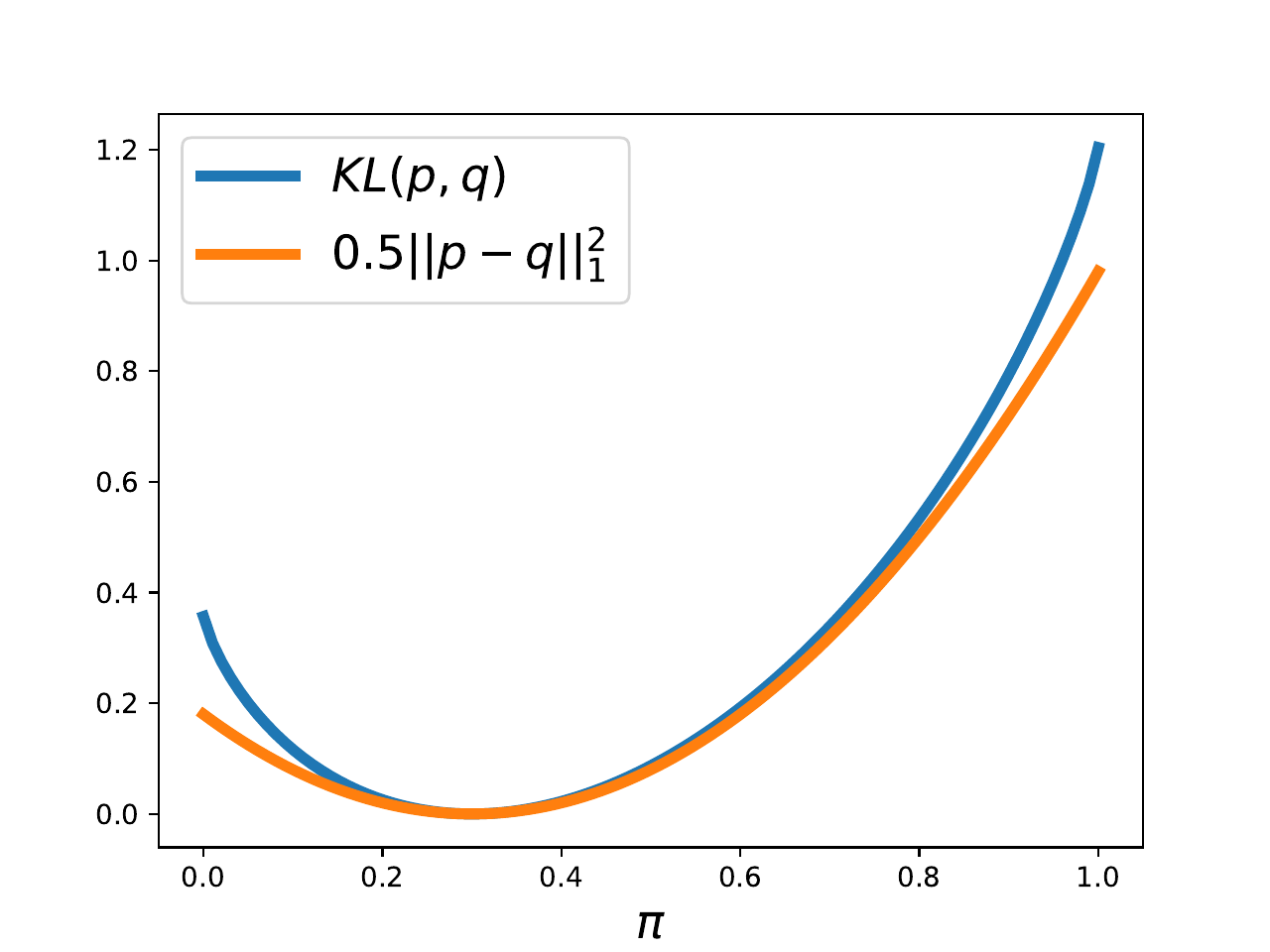
Figure 15.1: Graphical verification of Pinsker’s inequality, $\frac{1}{2} \|\p - \q\|_1^2 \le \mathrm{KL}(\p, \q)$ , with $\p \coloneqq (\pi, 1-\pi)$ and $\q \coloneqq (0.3, 0.7)$ .

15.4.5 Nonconvex functions

In general, the minimum of a function necessarily has a null gradient, that is, $\w^\star \in \argmin_{\w \in \cW} L(\w) \implies \nabla L(\w^\star) = 0.$ To see this, consider the function $F: t \rightarrow L(\w^\star - t \nabla L(\w^\star))$ . If $\nabla L(\w^\star)\neq 0$ , then $F'(0) = -\|\nabla L(\w^\star)\|_2^2 \neq 0$ . Therefore, there exists a small $t >0$ such that $F(t) < F(0)$ , i.e., $L(\w^\star)$ is not the minimum. However, if the function is not convex, the converse is a priori not true: finding a point that has a null gradient does not ensure that we have found a global minimum as illustrated in Figure 15.3.

For non-convex functions, a point with null gradient is called a stationary point. A stationary point may define a local maximum or a local minimum. Formally, $\hat \w$ is a local minimum if $\exists r>0, \ \mbox{s.t.}\ \forall \v \in \cW\ \mbox{satisfying} \ \|\v-\hat \w\|\leq r, \ \mbox{we have} \ L(\v) \geq L(\hat\w).$ A local maximum is defined similarly, except that $L(\v) \leq L(\hat\w)$ in a neighborhood of $\hat \w$ . For non-convex functions, convergence rates are therefore generally expressed in terms of convergence of the norm of the gradient $\|\nabla L(\w \pow t)\|_2$ towards $0$ . Such theoretical results do not ensure convergence to the global minimum but rather convergence to a point where no further progress may a priori be possible with just gradient information.

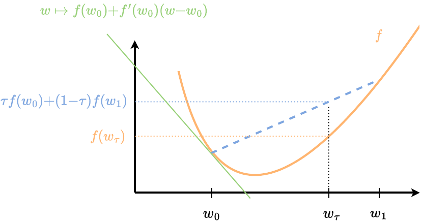
Figure 15.2: Convex function: any secant is above the function, any tangent is below the function, a point with zero gradient is a minimum.

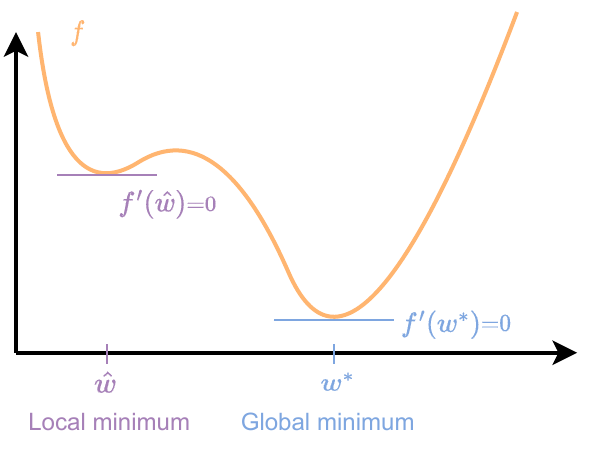
Figure 15.3: Non-convex function: a point with zero gradient is not necessarily the global minimum.

15.5 Performance guarantees

For a given class of functions, we can define the performance of an algorithm as the number of iterations the algorithm would need to find an $\varepsilon$ -accurate solution as in Eq. (15.1). This is called the computational complexity of the algorithm, denoted $t = T(\varepsilon).$ Alternatively, the performance of an algorithm can be stated in terms of convergence rate, i.e., the accuracy that the algorithm reaches after $t$ iterations, $\varepsilon = R(t),$ where $R$ is a decreasing positive function vanishing as $t \rightarrow +\infty$ . Usually, $R$ incorporates properties of the function minimized, such as its smoothness constant $\beta$ and information on the initial point, such as its function value. The corresponding computational complexity $T(\varepsilon)$ is then given as the minimum number of iterations $t$ such that $R(t) \leq \varepsilon$ , $T(\varepsilon) = \min \{t \in \NN \colon R(t) \le \varepsilon\}.$

Convergence rates can generally be classified by considering the progress ratio on iteration $t$ , defined by $\rho_t \coloneqq \frac{R(t)}{R(t-1)}.$ The asymptotic convergence rate is then defined by $\rho_{\infty} \coloneqq \lim_{t \rightarrow + \infty} \rho_t.$ We can classify the rates as follows.

Sublinear convergence rates, $\rho_\infty =1$ : the longer the algorithm runs, the slower it makes progress. That is, the relative progress eventually tends to stall as $t \rightarrow + \infty$ . Examples of $R(t)$ in this category include $O(1/t), O(1/t^2)$ or more generally $O(1/t^\alpha)$ for some $\alpha>0$ . This is equivalent to $T(\varepsilon) = O(\varepsilon^{-1/\alpha})$ .
Linear convergence rates, $\rho_\infty = c \in (0, 1)$ : the algorithm eventually reaches a state of constant relative progress at each iteration, leading to an overall rate $R(t) = O(\exp(- c t))$ for $c$ depending on the properties of the objective. This corresponds to $T(\varepsilon) = O (c^{-1}\ln \varepsilon^{-1})$ .
Superlinear convergence rates, $\rho_\infty = 0$ : the relative progress is better at each new iteration. This can happen for, e.g., $R(t) = O(\exp(-t^2))$ , leading to $T(\varepsilon) = O( \sqrt{\ln\varepsilon^{-1}})$ , or $R(t) = O(\exp(-2^t))$ , which is specifically called a quadratic rate, leading to $T(\varepsilon) = O (\ln\ln\varepsilon^{-1})$ .

This is illustrated in Fig. 15.4.

Note that the term “linear” may be misleading as the rates are in fact exponential. They are called “linear” because of their behavior in log scale.

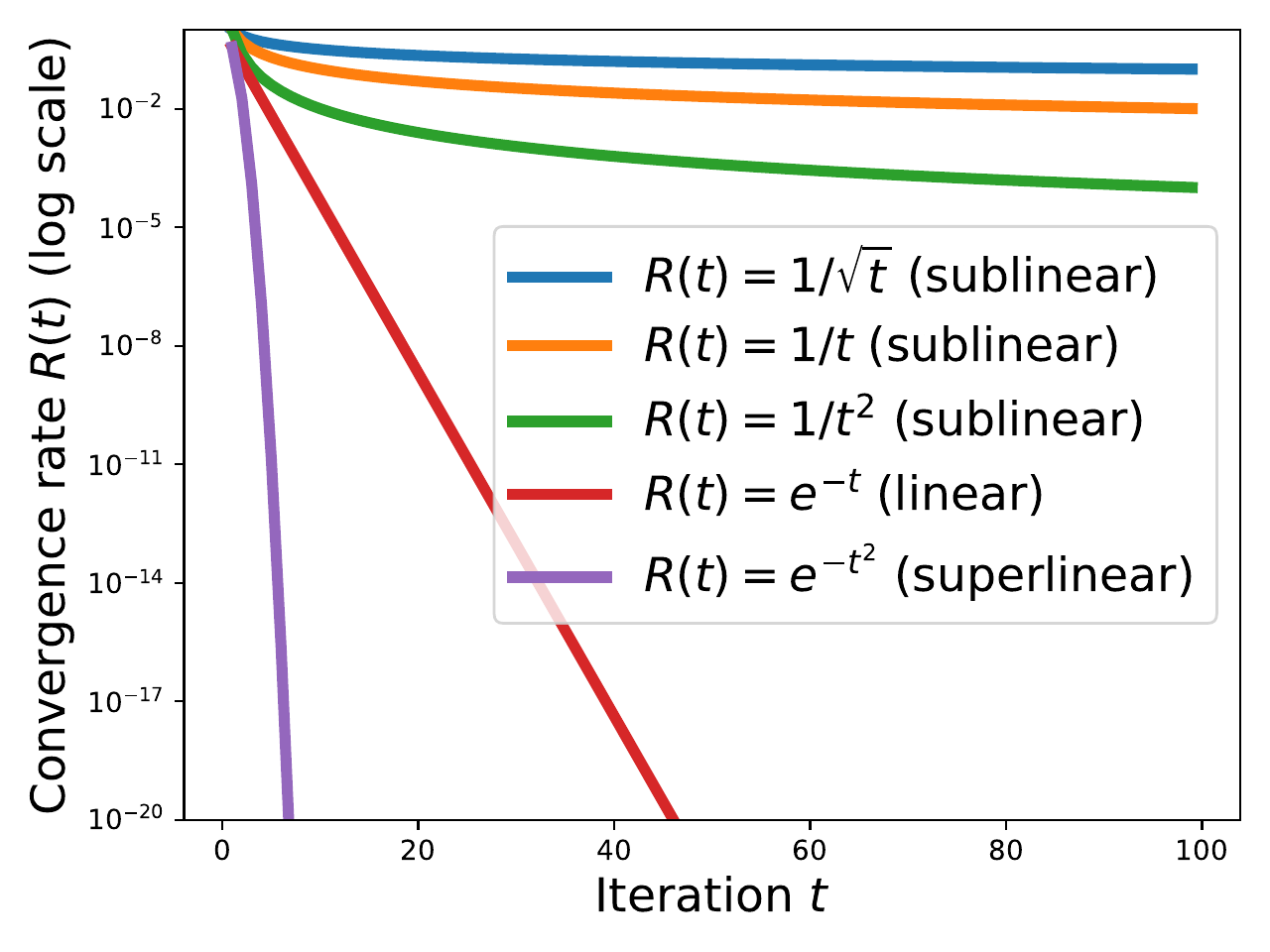
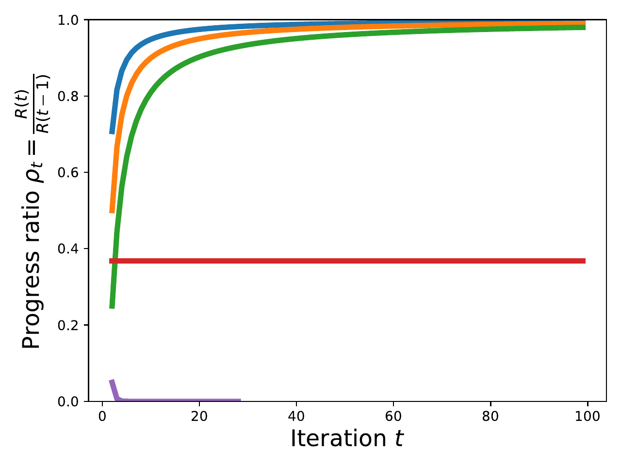
Figure 15.4: Left: convergence rates. Right: progress ratios. An algorithm with sublinear convergence rates eventually stops making progress. An algorithm with linear convergence rate eventually reaches a state of constant progress. An algorithm with superlinear convergence rate makes faster progress after each iteration.

Upper and lower bounds

The best performance of a class of algorithms equipped with a given oracle (e.g. first-order oracle) can be upper-bounded or lower-bounded. This allows to show that an algorithm with access limited to a certain type of oracle cannot theoretically do better than a certain number. For example, the computational complexity to minimize $\beta$ -smooth functions restricted on $[0, 1]^P$ with first-order oracles is lower bounded by $\frac{c}{\varepsilon^P}$ (Nemirovski and Yudin, 1983, p. 1.1.7). For example, with $P = 10$ and $\varepsilon=10^{-3}$ , this gives $10^{30}$ iterations. Note that these results are pessimistic by construction. The actual performance of an algorithm on a specific instance of this function class may be much better than this worst-case scenario, as it is the case with popular algorithms such as quasi-Newton methods. Better computational complexities can be achieved by further restricting the class of functions to the set of convex functions, which play a central role in optimization and many other fields.

Zero-order vs. first-order

For the class of smooth strongly convex functions, the computational complexity of the best first-order algorithm is (up to constant and logarithmic factors) $P$ times better than that of the best zero-order algorithm (Nesterov, 2018; Nesterov and Spokoiny, 2017). This theoretical comparison shows that, while zero-order optimization algorithms may perform on par with first-order optimization algorithms for problems with a low dimension $P$ , they can be much slower for high dimensional problems, i.e., $P\gg 1$ .

In different settings, for example with stochastic oracles (Duchi et al., 2015) or for different classes of functions, slightly different comparisons may be achieved, such as a $\sqrt{P}$ factor instead of $P$ . However, the same conclusion holds in the current frameworks considered: first-order optimization algorithms can provide fast rates that are dimension independent while the rates of zero-order optimization algorithms generally depend on the dimension of the problem, making them unfit for high-dimensional problems.

This explains the immense success of first-order algorithms for training neural networks. Fortunately, using reverse-mode autodiff, as studied in Chapter 8, it can be shown that computing a gradient has roughly the same complexity as evaluating the function itself Section 8.3.3.

15.6 Summary

The information available to us on a function can be formalized by the notion of oracle. Zero-order oracles can only evaluate the function; first-order oracles can also compute the gradient; second-order oracles can also compute the Hessian or the Hessian-vector product (HVP).
Most optimization algorithms reviewed in this book can be viewed from a variational perspective, in which the next iteration is produced by optimizing a trade-off between an approximation of the function and a proximity term. Different approximations and different proximity terms lead to different algorithms.
We also reviewed different classes of functions, and performance guarantees.