Chapter 14Smoothing by integration

In this chapter, we review smoothing techniques based on convolution.

14.1 Convolution

14.1.1 Convolution operators

The convolution between two functions $f$ and $g$ produces another function, denoted $f \ast g$ . It is defined by $(f \ast g)(\mu) \coloneqq \int_{-\infty}^\infty f(u) g(\mu - u) \, du, \tag{14.1}$ assuming that the integral is well-defined. It is therefore the integral of the product of $f$ and $g$ after $g$ is reflected about the $y$ -axis and shifted. It can be seen as a generalization of the moving average. Using the change of variable $u \coloneqq \mu + z$ , we can also write $\begin{aligned} (f \ast g)(\mu) &= \int_{-\infty}^\infty f(\mu + z) g(-z) \, dz \\ &= \int_{\infty}^{-\infty} f(\mu - v) g(v) \, (-dv) \\ &= \int_{-\infty}^\infty g(v) f(\mu - v) \, dv \\ &= (g \ast f)(\mu). \end{aligned} \tag{14.2}$ The convolution operator is therefore commutative.

Remark 14.1 (Change of variables)

Readers with a background in signal processing might find the change of variables $u \coloneqq \mu + z$ slightly unconventional for proving the commutativity of the convolution, as $u \coloneqq \mu - z$ more directly proves commutativity. However, we intentionally use $u \coloneqq \mu + z$ here, as this perfectly aligns our notation with the location-scale transform $U \coloneqq \muv + \sigma Z$ from Section 12.4.1. It allows us to seamlessly interpret smoothing by convolution as the injection of additive noise.

14.1.2 Convolution with a kernel

The convolution is frequently used together with a kernel $\kappa$ to create a smooth approximation $f \ast \kappa$ of $f$ . The most frequently used kernel is the Gaussian kernel with width $\sigma$ , defined by $\kappa_\sigma(z) \coloneqq \frac{1}{\sqrt{2\pi}\sigma} e^{-\frac{1}{2}(\frac{z}{\sigma})^2}.$ This is the probability density function (PDF) of the normal distribution with zero mean and variance $\sigma^2$ . The term $\frac{1}{\sqrt{2\pi}\sigma}$ is a normalization constant, ensuring that the kernel sums to $1$ for all $\sigma$ . We therefore say that $\kappa_\sigma$ is a normalized kernel.

Averaging perspective

Applying the definition of the convolution in Eq. (14.1), we obtain $\begin{align*} (f \ast \kappa_\sigma)(\mu) &\coloneqq \frac{1}{\sqrt{2\pi}\sigma} \int_{-\infty}^\infty f(u) e^{-\frac{1}{2} (\frac{\mu - u}{\sigma})^2} du \\ &= \EE_{U \sim p_{\mu,\sigma}}[f(U)], \end{align*}$ where $p_{\mu,\sigma}(u) \coloneqq \kappa_\sigma(\mu - u) = \frac{1}{\sqrt{2\pi}\sigma} e^{-\frac{1}{2} (\frac{\mu - u}{\sigma})^2}$ is the PDF of the Gaussian distribution with mean $\mu$ and variance $\sigma^2$ . Therefore, we can see $f \ast \kappa_\sigma$ as the expectation of $f(u)$ over a Gaussian centered around $\mu$ . This property is true for all translation-invariant kernels, that correspond to a location-scale family distribution (e.g., the Laplace distribution). The convolution therefore performs an averaging with all points, with points nearby $\mu$ given more weight by the distribution. The parameter $\sigma$ controls the importance we want to give to farther points. We call this viewpoint averaging, as we replace $f(u)$ by $\EE[f(U)]$ .

Perturbation perspective

Conversely, using the alternative definition of the convolution operator in Eq. (14.2), which stems from the commutativity of the convolution, we have $\begin{align*} (f \ast \kappa_\sigma)(\mu) &\coloneqq \int_{-\infty}^\infty f(\mu + z) e^{-\frac{1}{2} (\frac{-z}{\sigma})^2} dz \\ &= \int_{-\infty}^\infty f(\mu + z) e^{-\frac{1}{2} (\frac{z}{\sigma})^2} dz \\ &= \EE_{Z \sim p_{0,\sigma}}[f(\mu + Z)], \end{align*}$ where, in the second line, we used that the Gaussian kernel $p_{0,\sigma}$ is sign invariant, i.e., $p_{0,\sigma}(-z) = p_{0,\sigma}(z)$ . This viewpoint shows that smoothing by convolution with a Gaussian kernel can also be seen as injecting Gaussian noise or perturbations to the function’s input.

Limit case

When $\sigma \to 0$ , the kernel $\kappa_\sigma$ converges to a Dirac delta function, $\lim_{\sigma \to 0} \kappa_\sigma(z) = \delta(z).$ Since the Dirac delta is the multiplicative identity of the convolution algebra (this is also known as the sifting property), when $\sigma \to 0$ , $f \ast \kappa_\sigma$ converges to $f$ , i.e., $\lim_{\sigma \to 0} (f \ast \kappa_\sigma)(u) = f(u).$

14.1.3 Discrete convolution

Many times, we work with functions whose convolution does not have an analytical form. In these cases, we can use a discrete convolution on a grid of values. For two functions $f$ and $g$ defined over $\ZZ$ , the discrete convolution is defined by $(f \ast g)[i] \coloneqq \sum_{j=-\infty}^\infty f[j] g[i - j].$ As for its continuous counterpart, the discrete convolution is commutative, namely, $(f \ast g)[i] = \sum_{j=-\infty}^\infty f[i - j] g[j] = (g \ast f)[i].$ When $g$ has finite support over the set $S \coloneqq \{-M, -M+1, \dots, 0, \dots, M-1, M\}$ , meaning that $g[i] = 0$ for all $i \not \in S$ , a finite summation may be used instead, i.e., $(f \ast g)[i] = \sum_{j=-M}^M f[i - j] g[j] = (g \ast f)[i].$

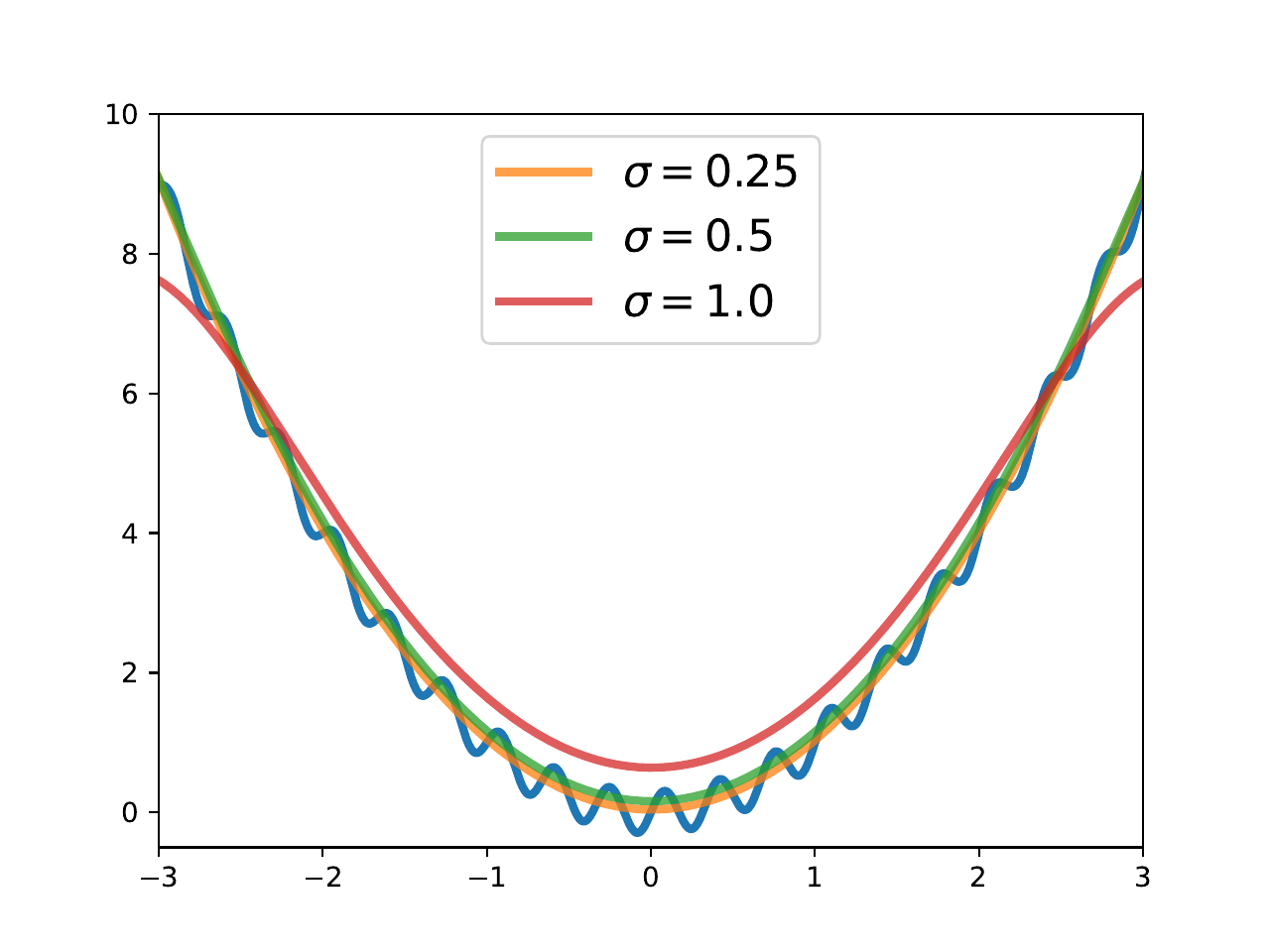
In practice, convolution between a discrete signal $f \colon \ZZ \to \RR$ and a continuous kernel $\kappa \colon \RR \to \RR$ is implemented by discretizing the kernel. One of the simplest approaches consists in sampling points on an interval, evaluating the kernel at these points and renormalizing the obtained values, so that the sampled kernel sums to $1$ . This is illustrated with the Gaussian kernel in Fig. 14.1. Since the Gaussian kernel decays exponentially fast, we can choose a small interval around $0$ . For a survey of other possible discretizations of the Gaussian kernel, see Getreuer (2013).

Figure 14.1: Smoothing of the signal $f[t] \coloneqq t^2 + 0.3 \sin(6\pi t)$ with a sampled and renormalized Gaussian kernel.

14.1.4 Differentiation

Remarkably, provided that the two functions are integrable with integrable derivatives, the derivative of the convolution satisfies $(f \ast g)' = (f' \ast g) = (f \ast g'),$ which simply stems from switching derivative and integral in the definition of the convolution. Moreover, we have the following proposition.

Proposition 14.1 (Differentiability of the convolution)

If $g$ is $n$ -times differentiable with compact support over $\RR$ and $f$ is locally integrable over $\RR$ , then $f \ast g$ is $n$ -times differentiable over $\RR$ .

14.1.5 Multidimensional convolution

So far, we studied the convolution of one-dimensional functions. The definition can be naturally extended to multidimensional functions $f \colon \RR^M \to \RR$ and $g \colon \RR^M \to \RR$ as $(f \ast g)(\muv) \coloneqq \int_{\RR^M} f(\u) g(\muv - \u) \, d\u,$ assuming again that the integral exists. Typically, a Gaussian kernel with diagonal covariance matrix is used $\begin{align*} \kappa_\sigma(\z) &\coloneqq \prod_{j=1}^M \frac{1}{\sqrt{2\pi}\sigma_j} e^{-\frac{1}{2}(\frac{z_j}{\sigma_j})^2} = \frac{1}{\sqrt{2\pi}^M\sigma^M} e^{-\frac{1}{2}\frac{\|\z\|^2_2}{\sigma^2}}, \tag{14.3}\end{align*}$ where, in the second equality, we assumed $\sigma_1 = \dots = \sigma_M$ . In an image processing context, where $M=2$ , it is approximated using a discrete convolution and it is called a Gaussian blur.

14.1.6 Link between convolution and infimal convolution

The infimal convolution we studied in Section 13.1 takes the form $(f \square g)(\muv) \coloneqq \inf_{\u \in \RR^M} f(\u) + g(\muv - \u).$ In comparison, the classical convolution takes the form $(F \ast G)(\muv) \coloneqq \int_{\RR^M} F(\u) G(\muv - \u) \, d\u.$ The two forms of convolution are clearly related. Infimal convolution performs an infimum and uses the sum of $f$ and $g$ : it uses a min-plus algebra. Classical convolution performs an integral and uses the product of $F$ and $G$ : it uses a sum-product algebra.

14.1.7 The soft infimal convolution

The link between the infimal convolution and the classical convolution can be further elucidated if we replace the infimum with a soft minimum in the definition of the infimal convolution.

Definition 14.1 (Soft infimal convolution)

The soft infimal convolution between $f \colon \RR^M \to \RR$ and $g \colon \RR^M \to \RR$ is $(f \square_\varepsilon g)(\muv) \coloneqq \underset{\u \in \RR^M}{\mathrm{softmin}_\varepsilon} ~ f(\u) + g(\muv - \u),$ where we defined the soft minimum (assuming that it exists) over $\cS$ of any function $h \colon \cS \to \RR$ as $\underset{\u \in \cS}{\mathrm{softmin}_\varepsilon} ~ h(\u) \coloneqq -\varepsilon \log \int_{\cS} \exp\left(-h(\u) / \varepsilon \right) d\u.$

We recover the infimal convolution as $\varepsilon \to 0$ .

Computation using a convolution

We now show that we can rewrite the soft infimal convolution using a classical convolution. Indeed, by using the exponential change of variable (sometimes referred to as Cole-Hopf transformation in a partial differential equation context) $\begin{align*} \cC_\varepsilon\{f\}(\u) &\coloneqq \exp(-f(\u) / \varepsilon) \\ \cC_\varepsilon^{-1}\{F\}(\v) &= -\varepsilon \log F(\v), \end{align*}$ we can define each function in the exponential domain, $\begin{align*} F_\varepsilon &\coloneqq \cC_\varepsilon\{f\} \\ G_\varepsilon &\coloneqq \cC_\varepsilon\{g\} \\ H_\varepsilon &\coloneqq \cC_\varepsilon\{h_\varepsilon\}. \end{align*}$ It is easy to check that we then have $H_\varepsilon(\muv) = (F_\varepsilon \ast G_\varepsilon)(\muv).$ Back to log domain, we obtain $h_\varepsilon(\muv) = \cC_\varepsilon^{-1}\{H_\varepsilon\}(\muv).$ Combining the transformation and its inverse, we can write $\begin{align*} h_\varepsilon(\muv) = \cC_\varepsilon^{-1}\{\cC_\varepsilon\{f\} \ast \cC_\varepsilon\{g\}\}(\muv). \end{align*}$ What we have shown is that, after an exponential change of variable, the soft infimal convolution can be reduced to the computation of a convolution. This is useful as a discrete convolution on a grid of size $n$ can be computed in $O(n \log n)$ .

14.1.8 The soft Moreau envelope

We saw in Section 13.1.2 that the infimal convolution between $f$ and $R(z) = \frac{1}{2} z^2$ is the Moreau envelope, $M_f(\muv) \coloneqq (f \square R)(\muv) = \inf_{\u \in \RR^M} f(\u) + \frac{1}{2} \|\muv - \u\|^2_2.$ Replacing the infimal convolution with a soft infimal convolution, we can define the “soft” Moreau envelope, $M_f^\varepsilon(\muv) \coloneqq (f \square_\varepsilon R)(\muv) = \underset{\u \in \RR^M}{\mathrm{softmin}_\varepsilon} ~ f(\u) + \frac{1}{2} \|\muv - \u\|^2_2.$ We emphasize that this operation is not the same as the convolution of $f$ with a Gaussian kernel. Indeed, we have $\begin{align*} M_f^\varepsilon(\muv) = -\varepsilon \log \int_{\RR^M} \exp\left((-f(\u) - \frac{1}{2} \|\muv - \u\|_2^2) / \varepsilon \right) d\u. \end{align*}$ while $\begin{align*} (f \ast \kappa_\sigma)(\muv) \coloneqq \int_{\RR^M} f(\u) \kappa_\sigma(\muv - \u) \, d\u, \end{align*}$ where $\kappa_\sigma$ is for instance defined in Eq. (14.3).

We saw that the Moreau envelope is a smooth function. One may therefore ask what do we gain from using a soft Moreau envelope. The benefit can be computational, as the latter can be approximated using a discrete convolution.

14.2 Fourier and Laplace transforms

Let us define the Fourier transform of $f$ by $F(s) \coloneqq \cF\{f\}(s) \coloneqq \int_{-\infty}^{\infty}f(t) e^{-i 2 \pi s t} \, dt, \quad s \in \RR.$ Note that $\cF\{f\}$ is a function transformation: it transforms $f$ into another function $F$ .

14.2.1 Convolution theorem

Now, consider the convolution $h(t) \coloneqq (f \ast g)(t).$ If we define the three transformations $\begin{align*} F &\coloneqq \cF\{f\}, \ G \coloneqq \cF\{g\}, \ H \coloneqq \cF\{h\}, \end{align*}$ the convolution theorem states that $H(s) = F(s) \cdot G(s), \quad s \in \RR.$ Written differently, we have $\cF\{f \ast g\} = \cF\{f\} \cdot \cF\{g\}.$ In words, in the Fourier domain, the convolution operation becomes a multiplication. Conversely, $h(t) = (f*g)(t) = \cF^{-1}\{F \cdot G\}(t), \quad t \in \RR.$ The convolution theorem also holds if we replace the Fourier transform with the Laplace transform or with the two-sided (bilateral) Laplace transform.

14.2.2 Link between Fourier and Legendre transforms

In Section 13.2, we studied another function transformation: the convex conjugate, also known as Legendre-Fenchel transform. We recap the analogies between these transforms in Table 14.1. In particular, the counterpart of $\cF\{f \ast g\} = \cF\{f\} \cdot \cF\{g\}$ for the infimal convolution is $(f \square g)^* = f^* + g^*.$ In words, the Legendre-Fenchel transform is to the infimal convolution what the Fourier transform is to the convolution.

Table 14.1: Analogy between Fourier and Legendre transforms. See Proposition 13.3 for more conjugate calculus rules.

	Fourier $\cF\{f\}$	Legendre $f^*$
Semiring	$(+, \cdot)$	$(\min, +)$
Scaling $(a > 0)$	$f(t) = g(t / a)$	$f(t) = a g(t/a)$
	$\cF\{f\}(s) = a\cF\{g\}(as)$	$f^(s) = a g^(s)$
Translation	$f(t) = g(t - t_0)$	$f(t) = g(t - t_0)$
	$\cF\{f\}(s) = e^{-i 2 \pi t_0 s} \cF\{g\}(s)$	$f^(s) = g^(s) + t_0$
Convolution	$h = f \ast g$	$h = f \square g$
	$\cF\{h\} = \cF\{f\} \cdot \cF\{g\}$	$h^* = f^* + g^*$
Gaussian / quadratic	$f(t) = e^{-at^2}$	$f(t) = \frac{a}{2} t^2$
	$\cF\{f\}(s) = \sqrt{\frac{\pi}{a}} e^{-\pi^2 s^2/a}$	$f^*(s) = \frac{1}{2a} s^2$
Smoothing	$f \ast \kappa_\sigma$	$f \square \frac{1}{2\varepsilon} \\|\cdot\\|^2_2$

14.2.3 The soft Legendre-Fenchel transform

We saw in Section 13.2 that the Legendre-Fenchel transform (convex conjugate) of a function $f \colon \RR^M \to \RR$ is $f^*(\v) \coloneqq \max_{\u \in \RR^M} ~ \langle \u, \v \rangle - f(\u).$ If necessary, we can support constraints by including an indicator function in the definition of $f$ . The conjugate can be smoothed out using a log-sum-exp, which plays the role of a soft maximum (Section 13.5).

Definition 14.2 (Soft convex conjugate)

$f^*_\varepsilon(\v) \coloneqq \underset{\u \in \RR^M}{\mathrm{softmax}_\varepsilon} ~ \langle \u, \v \rangle - f(\u),$ where we defined the soft maximum (assuming that it exists) over $\cS$ of any function $g \colon \cS \to \RR$ as $\underset{\u \in \cS}{\mathrm{softmax}_\varepsilon} ~ g(\u) \coloneqq \varepsilon \log \int_{\cS} \exp\left(g(\u) / \varepsilon \right) d\u.$

In the limit $\varepsilon \to 0$ , we recover the convex conjugate.

Computation using a convolution

We now show that this smoothed conjugate can be rewritten using a convolution if we apply a bijective transformation to $f$ .

Proposition 14.2 (Smoothed convex conjugate as convolution)

The smoothed conjugate can be rewritten as $f^*_\varepsilon(\v) = \cQ_\varepsilon^{-1}\left\{\frac{1}{\cQ_\varepsilon\{f\} \ast G_\varepsilon}\right\}\left(\v\right)$ where $\begin{align*} G_\varepsilon &\coloneqq \cC_\varepsilon\left\{\frac{1}{2} \|\cdot\|^2_2\right\} = \exp\left(-\frac{1}{2} \frac{\|\cdot\|^2_2}{\varepsilon}\right) \\ \cQ_\varepsilon\{f\} &\coloneqq \cC_\varepsilon\left\{f(\cdot) - \frac{1}{2} \|\cdot\|^2_2\right\} = \exp\left(\frac{1}{2\varepsilon} \|\cdot\|^2_2 - \frac{1}{\varepsilon}f(\cdot)\right) \\ \cQ_\varepsilon^{-1}\{F\} &\coloneqq \frac{1}{2} \|\cdot\|^2_2 - \varepsilon \log(F(\cdot)). \end{align*}$

This insight was tweeted by Gabriel Peyré in April 2020.

Proof

${\small \begin{aligned} f^\ast_\varepsilon(\v) &\coloneqq \varepsilon \log \int \exp\left(\frac{1}{\varepsilon} \langle \u, \v \rangle - \frac{1}{\varepsilon} f(\u)\right) d\u \\ &= \varepsilon \log \int \exp\left(-\frac{1}{2\varepsilon} \|\u - \v\|^2_2 + \frac{1}{2\varepsilon} \|\u\|^2_2 + \frac{1}{2\varepsilon}\|\v\|^2_2 - \frac{1}{\varepsilon} f(\u)\right) d\u \\ &= \varepsilon \log \int \exp\left(-\frac{1}{2\varepsilon} \|\u - \v\|^2_2 + \frac{1}{2\varepsilon} \|\u\|^2_2 - \frac{1}{\varepsilon} f(\u)\right) d\u + \frac{1}{2} \|\v\|^2_2 \\ &= \varepsilon \log \int G_\varepsilon(\v - \u) \cQ_\varepsilon\{f\}(\u) d\u + \frac{1}{2} \|\v\|^2_2 \\ &= \varepsilon \log (\cQ_\varepsilon\{f\} \ast G_\varepsilon)(\v) + \frac{1}{2} \|\v\|^2_2 \\ &= \frac{1}{2} \|\v\|^2_2 - \varepsilon \log \left(\frac{1}{\cQ_\varepsilon\{f\} \ast G_\varepsilon}\right)(\v) \\ &= \cQ_\varepsilon^{-1}\left\{\frac{1}{\cQ_\varepsilon\{f\} \ast G_\varepsilon}\right\}\left(\v\right) \end{aligned} }$ ◻

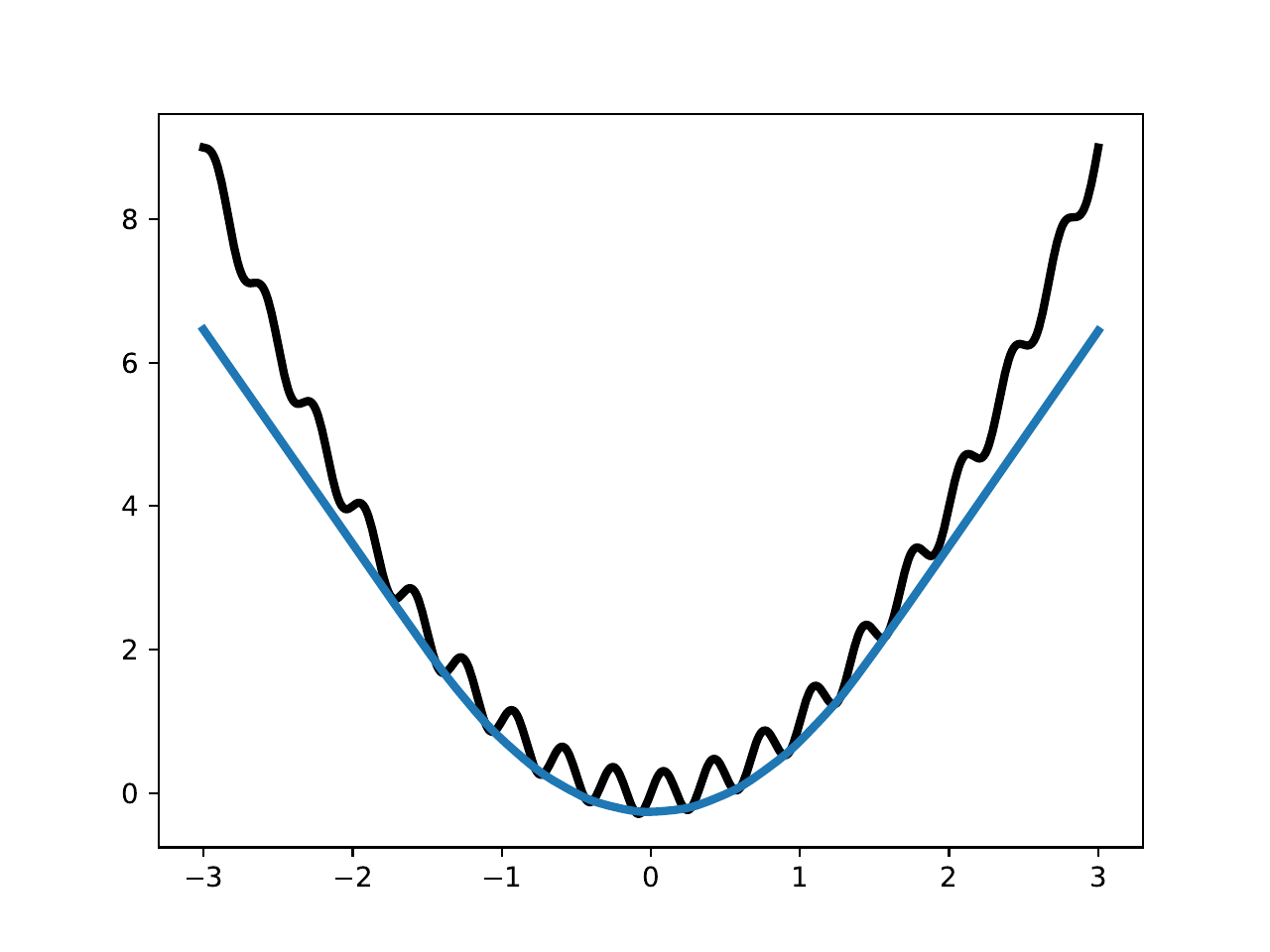
Figure 14.2: Applying the smoothed conjugate twice gives a smoothed biconjugate (convex envelope) of the function.

What did we gain from this viewpoint? The convex conjugate can often be difficult to compute in closed form. If we replace $\RR^M$ with a discrete set $\cS$ (i.e., a grid), we can then approximate the smoothed convex conjugate in $O(n \log n)$ , where $n = |\cS|$ , using a discrete convolution, $\begin{align*} (\cQ_\varepsilon\{f\} \ast G_\varepsilon)(\v) &\approx \sum_{\u \in \cS} G_\varepsilon(\v - \u) \cQ_\varepsilon\{f\}(\u) \\ &= \K \q, \end{align*}$ where $\K$ is the $n \times n$ Gaussian kernel matrix whose entries correspond to $\exp(-\frac{1}{2\varepsilon} \|\u - \u'\|^2_2)$ for $\u,\u' \in \cS$ and $\q$ is the $n$ -dimensional vector whose entries correspond to $\exp(\frac{1}{\varepsilon}(\frac{1}{2} \|\v\|^2_2 - f(\u))$ for $\u \in \cS$ . This provides a GPU-friendly alternative to the fast Legendre transform algorithm, discussed in Section 13.2. Of course, due to the curse of dimensionality, the technique is limited to functions defined on low-dimensional sets. We illustrate in Fig. 14.2 the application of the technique to computing an approximate biconjugate (convex envelope) of a function.

Remark 14.2 (Link with the two-sided Laplace transform)

For
one-dimensional functions, instead of using a convolution, we can also write the soft convex conjugate as $\begin{align*} f^*_\varepsilon(v) &= \varepsilon \log \int_{-\infty}^\infty \exp\left(\frac{1}{\varepsilon}\left[ uv - f(u)\right])\right) du \\ &= \varepsilon \log \cB\left\{e^{-\frac{f}{\varepsilon}}\right\}\left(-\frac{v}{\varepsilon}\right) \\ &= -\cC^{-1}_\varepsilon\left\{\cB\left\{\cC_\varepsilon\{f\}\right\}\right\} \left(-\frac{v}{\varepsilon}\right) \end{align*}$ where we defined the two-sided (bilateral) Laplace transform $\cB\{g\}(v) \coloneqq \int_{-\infty}^\infty e^{-uv} g(u) du$ and where we assumed that the integral exists.

14.3 Examples

In this section, we review practical examples for which the convolution with a Gaussian kernel enjoys an analytical solution.

14.3.1 Smoothed step function

Example 14.1 (Smoothed Heaviside)

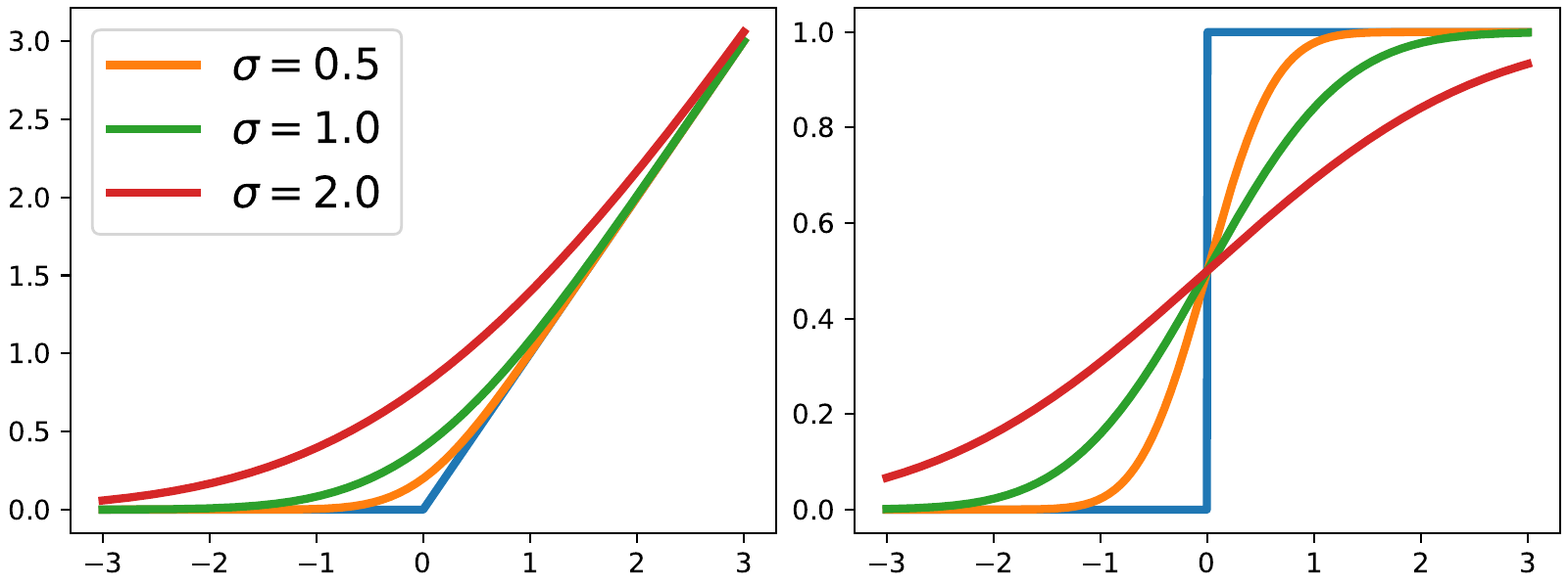
The Heaviside step function is defined by $\mathrm{step}(u) \coloneqq h(u) \coloneqq \begin{cases} 1 &\mbox{ if } u \ge 0 \\ 0 &\mbox{ otherwise} \end{cases}.$ With the Gaussian kernel, we therefore obtain $\begin{align*} (h \ast \kappa_\sigma)(\mu) &= \int_{-\infty}^\mu \kappa_\sigma(z) h(\mu - z) dz + \int_{\mu}^\infty \kappa_\sigma(z) h(\mu - z) dz \\ &= \int_{-\infty}^\mu \kappa_\sigma(z) dz \\ &= \Phi_\sigma(\mu) \\ &= \frac{1}{2} \left[1 + \mathrm{erf}\left(\frac{\mu}{\sqrt{2}\sigma}\right)\right], \end{align*}$ where $\Phi_\sigma(\mu)$ is the CDF of the Gaussian distribution with zero mean and variance $\sigma^2$ , and where we used the error function $\operatorname{erf}(z) \coloneqq \frac{2}{\sqrt\pi}\int_0^z e^{-t^2}\,\mathrm dt,$ that we both already encountered in Chapter 3. Although there is no closed form for the error function, it is commonly available in numerical analysis software, such as SciPy.

14.3.2 Smoothed ReLU function

Example 14.2 (Smoothed ReLU)

The ReLU is defined by $r(u) \coloneqq \begin{cases} u &\mbox{ if } u \ge 0 \\ 0 &\mbox{ otherwise} \end{cases} = u \cdot h(u).$ Similarly to the previous example, we obtain $\begin{align*} (r \ast \kappa_\sigma)(\mu) &= \int_{-\infty}^\mu \kappa_\sigma(z) r(\mu - z) dz \\ &= \int_{-\infty}^\mu \kappa_\sigma(z) (\mu - z) dz \\ &= \mu \int_{-\infty}^\mu \kappa_\sigma(z) dz - \int_{-\infty}^\mu \kappa_\sigma(z) z dz \\ &= \mu \Phi_\sigma(\mu) + \sigma^2 \kappa_\sigma(\mu). \end{align*}$ In the second integral, setting $a \coloneqq \frac{1}{2\sigma^2}$ , we used $\int z e^{-a z^2} dz = -\frac{1}{2a} \int e^t d t = -\frac{1}{2a} e^t + C = -\frac{1}{2a} e^{-a z^2} + C$ and $t \coloneqq -a z^2 \Rightarrow z dz = -\frac{1}{2a} d t$ .

Figure 14.3: Smoothing of the ReLU and Heaviside functions by convolution with a Gaussian kernel, for three values of the width $\sigma$ .

To illustrate differentiation of the convolution, we show how to differentiate the smoothed ReLU.

Example 14.3 (Differentiating the smoothed ReLU)

Differentiating the smoothed ReLU from Example 14.2, we obtain $(r \ast \kappa_\sigma)' = (r' \ast \kappa_\sigma) = h \ast \kappa_\sigma = \Phi_\sigma.$ Therefore, unsurprisingly, the derivative of the smoothed ReLU is the smoothed Heaviside step function. Differentiating once again, we obtain, $(r \ast \kappa_\sigma)'' = (h \ast \kappa_\sigma)' = (h' \ast \kappa_\sigma) = \delta \ast \kappa_\sigma = \kappa_\sigma,$ where the derivative $h'$ is well-defined almost everywhere. We can arrive at the same result by using that $h \ast \kappa_\sigma = \Phi_\sigma$ and $\Phi_\sigma' = \kappa_\sigma$ , since $\Phi_\sigma$ and $\kappa_\sigma$ are the CDF and PDF of the Gaussian with zero mean and $\sigma^2$ variance.

14.4 Perturbation of blackbox functions

In this section, we review how to approximately compute a convolution with a kernel and its gradient using Monte-Carlo estimation.

14.4.1 Expectation in a location-scale family

A rather intuitive approach to smooth a function $f: \RR^M\rightarrow \RR$ is to average its values on an input $\muv$ , perturbed by some additive noise $Z \sim p$ , for some noise distribution $p$ . This defines the surrogate $f_\sigma(\muv) \coloneqq \EE_{Z\sim p}[f(\muv + \sigma Z)].$ The parameter $\sigma$ controls the perturbation strength: as $\sigma \rightarrow 0$ , we naturally recover $f$ . An equivalent viewpoint is obtained by defining the transformation (change of variables) $U \coloneqq \muv + \sigma Z.$ We then have $U \sim p_{\muv, \sigma},$ where $p_{\muv, \sigma}$ is the location-family distribution generated by the noise distribution $p$ . It is the pushforward distribution of $Z$ through the transformation (see Section 12.4.4). In this notation, the initial noise distribution $p$ is then simply $p = p_{\zeros,1}$ . The perturbed function can then be expressed from these two perspectives as $\begin{align*} f_\sigma(\muv) &= \EE_{Z \sim p_{\zeros,1}}[f(\muv + \sigma \cdot Z)] \\ &= \EE_{U \sim p_{\muv,\sigma}}[f(U)]. \tag{14.4}\end{align*}$ Writing the expectation as the integral of a p.d.f, we naturally recover the smoothing by convolution presented earlier, $\begin{align*} f_\sigma(\muv) & = \int f(\muv + \sigma \z) p_{\zeros,1}(\z) d\z \\ & = f \ast \kappa_\sigma(\muv), \end{align*}$ where we defined the kernel $\kappa_\sigma(\z) \coloneqq p_{\zeros, \sigma}(-\z).$ In the sequel, we assume that the noise distribution decomposes as $p_{\zeros,1}(\z) \coloneqq \exp(-\nu(\z)) / C,$ where $\nu(\z)$ is the log-density of the noise distribution and $C$ is a normalization constant. For instance, the Gaussian distribution with diagonal covariance matrix and the corresponding Gaussian kernel are obtained with $\nu(\z) = \frac{1}{2} \|\z\|^2_2$ and $C=\sqrt{2\pi}^M$ .

Approximation by Monte-Carlo estimation

Instead of approximating the integral above (continuous convolution) with a discrete convolution on a grid, as we did in Section 14.1.3, the expectation perspective suggests that we can estimate $f_\sigma(\muv)$ by Monte-Carlo estimation: we simply draw samples from the distribution, evaluate the function at these samples and average. Beyond mere Monte-Carlo estimation, more elaborate approximation schemes are studied in (Chaudhuri and Solar-Lezama, 2010).

14.4.2 Gradient estimation by reparametrization

Provided that the conditions for swapping differentiation and integration hold (see Section 12.1), we have $\nabla f_\sigma(\muv) = \EE_{Z \sim p_{\zeros,1}}[\nabla f(\muv + \sigma \cdot Z)]. \tag{14.5}$ Note that if $f$ is only differentiable almost everywhere, the formula may still hold. For example, if $f$ is the ReLU, then $\nabla f$ is the Heaviside step function, and we obtain the correct gradient of $f_\sigma$ using the formula above; see Example 14.1. However, if $f$ is not absolutely continuous, the formula may not hold. For example, if $f$ is the Heaviside function, the right-hand side of (14.5) is 0 which does not match the gradient of $f_\sigma$ ; see again Example 14.1.

From the second expression of $f_{\sigma}$ in (14.4), we can see the formula of the gradient in (14.5) as a reparametrization trick $U = \muv+\sigma Z$ ; see Section 12.4. Namely, we have $\begin{align*} \nabla f_\sigma(\muv) &= \nabla_\muv \EE_{U \sim p_{\muv,\sigma}}[f(U)] \\ &= \nabla_\muv \EE_{Z \sim p_{\zeros,1}}[f(\muv + \sigma \cdot Z)] \\ &= \EE_{Z \sim p_{\zeros,1}}[\nabla_\muv f(\muv + \sigma \cdot Z)] \\ &= \EE_{Z \sim p_{\zeros,1}}[\nabla f(\muv + \sigma \cdot Z)]. \tag{14.6}\end{align*}$

14.4.3 Gradient estimation by SFE, Stein’s lemma

In some cases, we may not have access to $\nabla f$ or $f$ may not be absolutely continuous and therefore the formula in (14.5) cannot apply. For these cases, we can use the score function estimator (SFE) from Section 12.3. Here, for $f_\sigma(\muv) = \EE_{U \sim p_{\muv,\sigma}}[f(U)]$ , we obtain $\nabla f_\sigma(\muv) = \EE_{U \sim p_{\muv, \sigma}}[f(U) \nabla_{\muv} \log p_{\muv,\sigma}(U)].$ Since the PDF can be written as $p_{\muv,\sigma}(\u) = \frac{1}{\sigma} p_{\zeros,1}((\u - \muv) / \sigma),$ where $p_{\zeros,1}(\z) \coloneqq \exp(-\nu(\z)) / C,$ we obtain $\nabla_\muv \log p_{\muv,\sigma}(\u) = \nabla \nu((\u - \muv) / \sigma) / \sigma.$ To summarize, we have shown that $\begin{align*} \nabla f_\sigma(\muv) &= \EE_{U \sim p_{\muv, \sigma}}[f(U) \nabla \nu((U - \muv) / \sigma) / \sigma] \\ &= \EE_{Z \sim p_{\zeros, 1}}[f(\muv + \sigma \cdot Z) \nabla \nu(Z) / \sigma], \tag{14.7}\end{align*}$ where we used the change of variable $Z = (U - \muv) / \sigma$ . The same technique can also be used if we want to estimate the gradient w.r.t. $\thetav = (\muv, \sigma)$ or if we want to estimate the Jacobian of the expectation of a vector-valued function.

In the particular case of Gaussian noise, since $\nabla \nu(\z) = \z$ , we obtain $\begin{align*} \nabla f_\sigma(\muv) &= \EE_{Z \sim p_{\zeros, 1}}[f(\muv + \sigma \cdot Z) Z / \sigma]. \end{align*}$ This is known as Stein’s lemma. It should be noted that the above is an unbiased estimator of the gradient of the smoothed function $f_\sigma$ , but a biased estimator of the gradient of the original function $f$ (assuming that it exists). However, smoothing is usually a good thing, as it can accelerate the convergence of gradient-based algorithms. Computing the gradient of perturbed general programs is studied in detail in (Kreikemeyer and Andelfinger, 2023).

14.4.4 Link between reparametrization and SFE

Using the log-derivative identity, we have for any distribution with differentiable density $p$ $\begin{align*} \EE_{Z \sim p} [h(Z) \nabla \log p(Z)] &= \int_{\RR^M} h(\z) \left(\frac{\nabla p(\z)}{p(\z)}\right) p(\z) d\z \\ &= \int_{\RR^M} h(\z) \nabla p(\z) d\z. \end{align*}$ Using integration by parts and assuming that $h(\z)p(\z)$ goes to zero when $\|\z\| \to \infty$ , we have $\int_{\RR^M} h(\z) \nabla p(\z) d\z = -\int_{\RR^M} p(\z) \nabla h(\z) d\z.$ We have therefore the identity $\EE_{Z \sim p} [h(Z) \nabla \log p(Z)] = -\EE_{Z \sim p}[\nabla h(Z)].$ Importantly, contrary to the SFE estimator from Section 12.3, this identity uses gradients with respect to $\z$ , not with respect to the parameters of the distribution. Nevertheless, using the reparametrization $h(\z) \coloneqq f(\muv + \sigma \cdot \z)$ , we have $\nabla h(\z) = \nabla f(\muv + \sigma \cdot \z) \cdot \sigma$ so that $\begin{align*} \nabla f_\sigma(\muv) &= \nabla_\muv \EE_{U \sim p_{\muv,\sigma}}[f(U)] \\ &= \EE_{Z \sim p_{\zeros,1}}[\nabla f(\muv + \sigma \cdot Z)] \quad \text{(reparametrization trick)}\\ &= \EE_{Z \sim p_{\zeros,1}}[\nabla h(Z) / \sigma] \\ &= -\EE_{Z \sim p_{\zeros,1}}[h(Z) \nabla \log p(Z) / \sigma] \\ &= \EE_{Z \sim p_{\zeros,1}}[h(Z) \nabla \nu(Z) / \sigma] \\ &= \EE_{Z \sim p_{\zeros,1}}[f(\muv + \sigma \cdot Z) \nabla \nu(Z) / \sigma] \quad \text{(score function estimator)} \end{align*}$ Essentially, integration by parts allowed us to convert the reparametrization trick estimator into the SFE estimator. For more applications of integration by parts in machine learning, see Francis Bach’s excellent blog post.

14.4.5 Variance reduction and evolution strategies

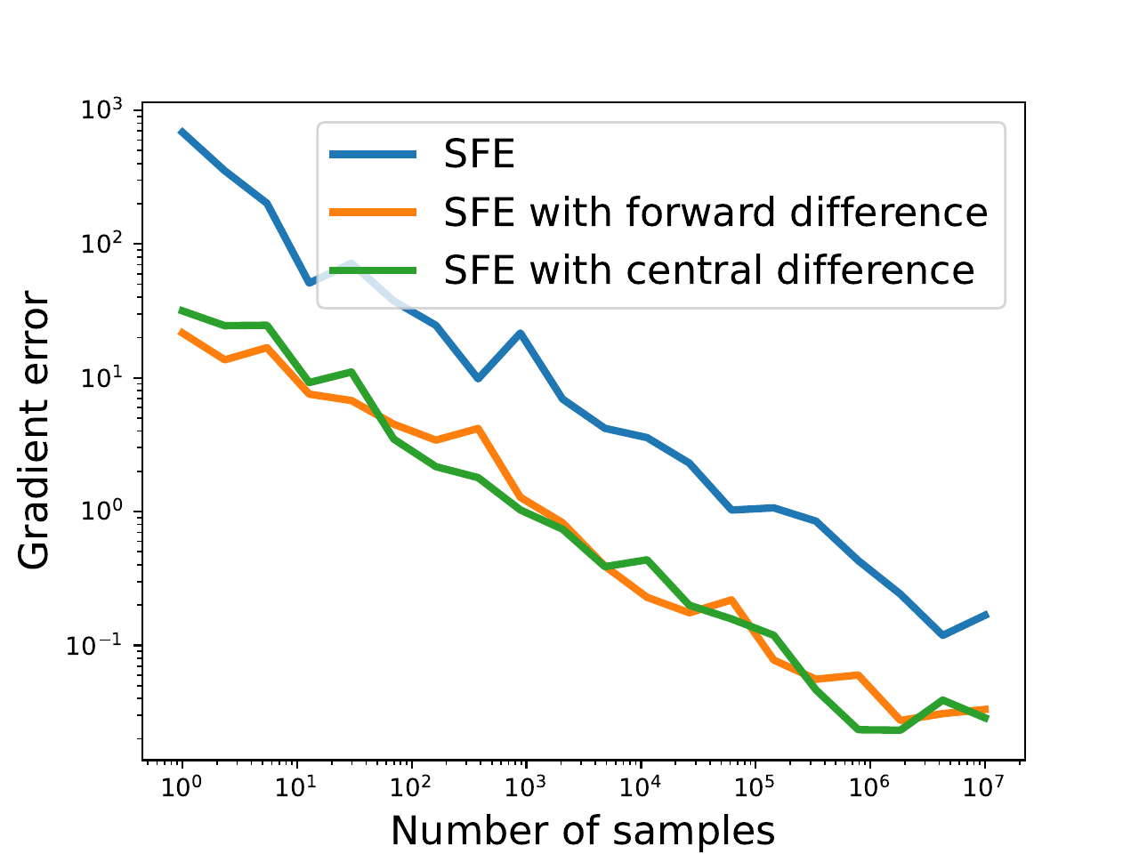
As discussed in Chapter 12, the SFE suffers from high variance. We now apply variance reduction techniques to it. To do so, we assume that $\nabla \nu(Z)$ has zero mean for $Z \sim p_{\zeros, 1}$ . This assumption for example holds for Gaussian noise. This assumption implies that $\EE_{Z \sim p_{\zeros, 1}}[f(\muv) \nabla \nu(Z) / \sigma] = f(\muv) \EE_{Z \sim p_{\zeros, 1}}[\nabla \nu(Z) / \sigma] = \zeros$ and therefore $\nabla f_\sigma(\muv) = \EE_{Z \sim p_{\zeros, 1}}\left[(f(\muv + \sigma \cdot Z) - f(\muv)) \nabla \nu(Z) / \sigma\right]. \tag{14.8}$ This is an example of control variate discussed in Section 12.3. This can be interpreted as using a finite difference for computing a directional derivative in the random direction $Z$ (see “limit case” below). Inspired by a central finite difference, we can also use $\nabla f_\sigma(\muv) = \EE_{Z \sim p_{\zeros, 1}}\left[(f(\muv + \sigma \cdot Z) - f(\muv - \sigma \cdot Z)) \nabla \nu(Z) / (2 \sigma)\right]. \tag{14.9}$ These estimators have been used as part of blackbox (zero-order) optimization algorithms, such as evolution strategies (Salimans et al., 2017) or random gradient-free optimization (Nesterov and Spokoiny, 2017). For quadratic functions, it is easy to show that the second estimator achieves lower variance (Recht and Frostig, 2017). The idea of sampling both $Z$ and $-Z$ simultaneously is called antithetic (Geweke, 1988) or mirrored sampling (Brockhoff et al., 2010). Evolution strategies have also been used to obtain unbiased gradient estimators of partially unrolled computational graphs (Vicol et al., 2021). We empirically compare the SFE with or without variance reduction for blackbox gradient estimation in Fig. 14.4.

Figure 14.4: Comparison of the score function estimator (SFE) with or without variance reduction for blackbox gradient estimation. We show the error $|\nabla f(\mu) - \nabla f_\sigma(\mu)|$ for $f(u) \coloneqq u^3$ and $f_\sigma(\mu) \coloneqq \EE[f(\mu + \sigma Z)]$ , where $Z \sim \mathrm{Normal}(0,1)$ and $\sigma \coloneqq 0.1$ . To estimate $\nabla f_\sigma(\mu)$ , we compare three estimators: the vanilla SFE Eq. (14.7), the SFE estimator with forward difference (variance reduced) Eq. (14.8), and the SFE estimator with central difference (variance reduced) Eq. (14.9). In all three cases, we approximate the expectation by Monte-Carlo estimation using some number of samples. The variance-reduced estimators not only achieve smaller error, they are also more numerically stable as $\sigma$ gets smaller.

14.4.6 Zero-temperature limit

We now discuss the limit case $\sigma \to 0$ . That is, we assume that we do not want to perform smoothing and that $\nabla f$ exists. We recall that the directional derivative of $f$ at $\muv$ in the direction $\z$ is $\begin{align*} \partial f(\muv)[\z] & = \langle \nabla f(\muv), \z \rangle \\ & = \lim_{\sigma \to 0} \left[f(\muv + \sigma \cdot \z) - f(\muv)\right] / \sigma. \end{align*}$ When $\sigma \to 0$ and $Z$ follows the standard Gaussian distribution, meaning that $\nabla \nu(\z) = \z$ , Eq. (14.8) therefore becomes $\begin{align*} \nabla f_\sigma(\muv) &= \EE_{Z \sim p_{\zeros, 1}} \left[\partial f(\muv)[Z] \nabla \nu(Z) \right] \\ &= \EE_{Z \sim p_{\zeros, 1}} \left[\partial f(\muv)[Z] Z \right] \\ &= \EE_{Z \sim p_{\zeros, 1}} \left[\langle \nabla f(\muv), Z \rangle Z\right] \\ &= \EE_{Z \sim p_{\zeros, 1}} \left[Z Z^\top \nabla f(\muv) \right] \\ &= \nabla f(\muv). \end{align*}$ This should not be too surprising, as we already know from the convolution perspective that $f_\sigma(\muv) = (f \ast \kappa_\sigma)(\muv) \to f(\muv)$ when $\sigma \to 0$ . This recovers the randomized forward-mode estimator already presented in Section 8.7.

14.5 Gumbel tricks

14.5.1 The Gumbel distribution

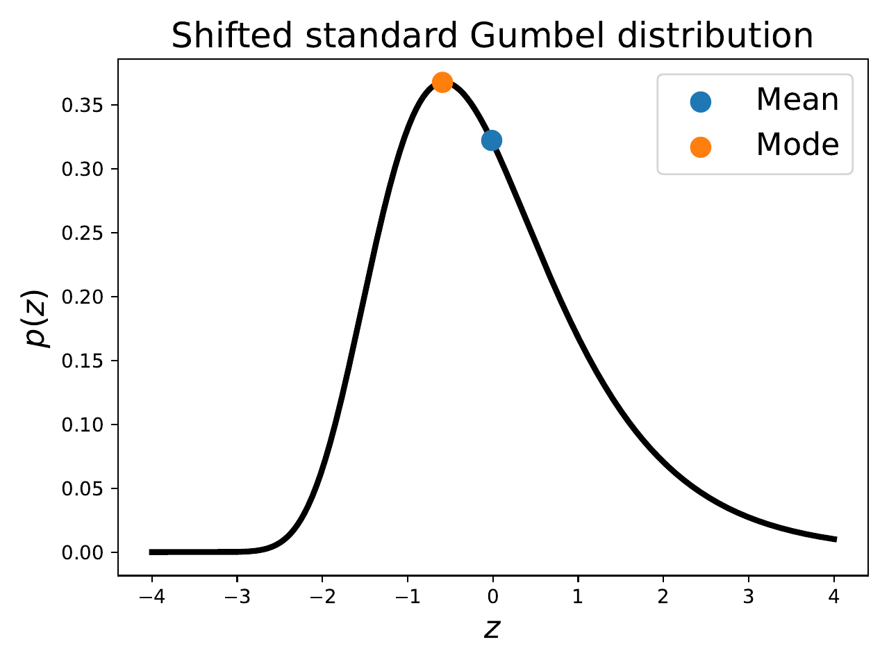
The Gumbel distribution is a distribution frequently used in extreme value theory. As illustrated in Fig. 14.5, we consider the shifted standard Gumbel distribution, whose PDF is defined by $p(z) \coloneqq \exp(-\nu(z)),$ where $\nu(z) \coloneqq z + \gamma + \exp(-(z+\gamma)),$ and where $\gamma \approx 0.577$ is Euler’s constant. Note that in some formulations, the distribution is not shifted, i.e., $\gamma$ is not added. If $Z$ is distributed according to the shifted standard Gumbel distribution, we write $Z \sim \mathrm{Gumbel}(0, 1)$ .

To obtain a multivariate extension with location-scale parameters $\muv$ and $\sigma$ , we take $M$ independent random variables $Z \coloneqq (Z_1, \ldots, Z_M)$ and apply the location-scale transform (Section 12.4.1). That is, $U \sim \mathrm{Gumbel}(\muv, \sigma) \iff U = \muv + \sigma Z, ~ Z_i \sim \mathrm{Gumbel}(0, 1).$ As we used shifted standard Gumbel distributions, we naturally get that $\EE[U] = \muv$ and $\Var(U) = \sigma^2$ . We can use Gumbel noise as an alternative to the Gaussian noise used in Section 14.4. Thankfully, in particular cases, we can compute closed-form expressions of the expectation of perturbed functions.

Remark 14.3 (Link between Gumbel and exponential distribution)

A random variable $Z$ is distributed as $\Gumbel(\mu, 1)$ if and only if $\exp(-Z)$ is distributed as an exponential distribution $\Exp(\exp(\mu - \gamma))$ . To see this, one can simply compute the CDF of $\exp(-Z)$ and recognize the CDF of $\Exp(\exp(\mu-\gamma))$ . Therefore, when comparing Gumbel distributions, we can use standard properties of the exponential distribution.

Remark 14.4 (Sampling Gumbel noise)

If $U \sim \mathrm{Uniform}(0,1)$ , then $Z \coloneqq -\log(-\log(U)) - \gamma$ satisfies $Z \sim \mathrm{Gumbel}(0, 1)$ , where we recall that we use $\mathrm{Gumbel}(0,1)$ to denote the shifted standard Gumbel distribution. To see this, note that $\PP(Z \leq t) = \PP(U \leq \exp(\exp(-(\gamma +t)))) = \exp(\exp(-(\gamma +t)))$ , where the last expression matches the CDF of $\mathrm{Gumbel}(0,1)$ .

Figure 14.5: We use a shifted definition of the standard Gumbel distribution so that the mean is achieved at $z = 0$ , and the mode at $z = -\gamma$ . With an unshifted definition, the mean and the mode would be achieved at $\gamma$ and $0$ , respectively.

14.5.2 Perturbed comparison

To start with, the Gumbel distribution can be used to smooth a binary comparison like the greater than or equal operators. Recall that the latter is defined for any $\mu_1, \mu_2 \in \RR$ as $\mathrm{gt}(\mu_1, \mu_2) \coloneqq \begin{cases} 1 & \mbox{if} \ \mu_1 \geq \mu_2 \\ 0 & \mbox{if} \ \mu_1 < \mu_2 \end{cases} = \heavistep(\mu_1-\mu_2),$ where $\heavistep$ is the Heaviside function. As shown below, by perturbing each variable with Gumbel noise, we recover $\logistic(a-b)= 1/(1+ e^{-(a-b)})$ as an approximation of $\heavistep(a-b)$ .

Proposition 14.3 (Gumbel trick for binary variables)

Let
$Z_1, Z_2 \sim \mathrm{Gumbel}(0,1)$ be two independent random variables. The difference of their location-scale transform (Section 12.4.1) is distributed according to a logistic distribution (Remark 3.1), i.e., $\mu_1 + \sigma Z_1 - (\mu_2 + \sigma Z_2) \sim \mathrm{Logistic}(\mu_1-\mu_2,\sigma),$ for $\mu_1, \mu_2 \in \RR$ and $\sigma >0$ . In particular, we have $\EE_{Z_1,Z_2}[\mathrm{gt}(\mu_1 + \sigma Z_1, \mu_2 + \sigma Z_2)] = \frac{1}{1+ e^{-(\mu_1-\mu_2)/\sigma}}.$

Proof

We first derive the CDF of $\mu_1 + \sigma Z_1 - (\mu_2 + \sigma Z_2)$ as $\begin{align*} \PP(\mu_1 + \sigma Z_1 - (\mu_2 + \sigma Z_2) \leq t) & = \PP\left(\mu_1/\sigma + Z_1 \leq (\mu_2 + t)/\sigma + Z_2\right) \\ & = \PP\left(e^{-(\mu_1/\sigma + Z_1)} \geq e^{-((\mu_2 + t)/\sigma + Z_2)}\right). \end{align*}$ By Remark 14.3, $e^{-(\mu_1/\sigma + Z_1)}\sim \Exp(\exp(\mu_1/\sigma - \gamma))$ , and similarly for $e^{-(\mu_2 + t)/\sigma + Z_2}$ . Now one easily shows that if $U \sim \Exp(u), V \sim \Exp(v)$ independent, then $\PP(U\leq V) = u/(u+v)$ . Hence, we get $\begin{align*} \PP(\mu_1 + \sigma Z_1 - (\mu_2 + \sigma Z_2) \leq t) & = \frac{e^{(\mu_2 + t)/\sigma - \gamma }}{e^{(\mu_2 + t)/\sigma - \gamma } + e^{\mu_1/\sigma - \gamma}} \\ & = \frac{1}{1+ e^{-(t- (\mu_1-\mu_2))/\sigma}}. \end{align*}$ We recognize the CDF of the logistic distribution with mean $\mu_1-\mu_2$ and scale $\sigma$ , denoted $\mathrm{Logistic}(\mu_1 - \mu_2, \sigma)$ . For the last claim, we simply have that $\begin{align*} \EE[\mathrm{gt}(\mu_1 + \sigma Z_1, \mu_2 + \sigma Z_2)] & = \EE\left[\heavistep(\mu_1+ \sigma Z_1 - (\mu_2+ \sigma Z_2))\right] \\ & = \PP(\mu_1 + \sigma Z_1 - (\mu_2 + \sigma Z_2)\geq 0) \\ & = \frac{1}{1+e^{-(\mu_1-\mu_2)/\sigma}}. \end{align*}$ ◻

14.5.3 Perturbed argmax

Suppose we want to smooth $\y(\u) \coloneqq \argmax_{\y \in \{\e_1, \dots, \e_M\}} \langle \y, \u \rangle = \phi(i(\u)),$ where $\begin{align*} i(\u) & \coloneqq \argmax_{i \in [M]} u_i \\ \phi(i) & \coloneqq \e_i \end{align*}$ where $\phi(i)$ is the one-hot encoding of $i \in [M]$ . It turns out that the function $\y(\u)$ perturbed using Gumbel noise enjoys a closed form expectation, which is nothing else than the softargmax.

Proposition 14.4 (Gumbel trick for categorical variables)

Let us define $M$ independent random variables $Z \sim \mathrm{Gumbel}(\zeros, 1) \in \RR^M$ . Then, for $\muv \in \RR^M$ and $\sigma >0$ , $Y \coloneqq i(\muv + \sigma \cdot Z) \implies Y \sim \mathrm{Categorical}(\mathrm{softargmax}(\muv / \sigma)).$ Moreover, we have $\begin{align*} \y_\sigma(\muv) & = \EE_Z[\y(\muv + \sigma \cdot Z)] \\ & = \EE_Y[\phi(Y)] \\ & = \mathrm{softargmax}(\muv / \sigma). \end{align*}$

Proof

For $k \in [M]$ , we have that $\begin{align*} \PP(Y = k) & = \PP\left(\argmax_{i \in [M]} \{\mu_i + \sigma Z_i\} = k\right) \\ & = \PP\left(\argmin_{i \in [M]} \{e^{-\mu_i/\sigma - Z_i} \} = k\right) \end{align*}$ By Remark 14.3, we have that $e^{-\mu_i/\sigma - Z_i} \sim \Exp(\exp(\mu_i/\sigma - \gamma))$ . One easily verifies as an exercise, that, for $U_1, \ldots, U_M$ independent exponential variables with parameters $u_1, \ldots, u_M$ , we have $\PP(\argmin_{i \in [M]} \{U_i\} = k) = u_k/\sum_{i=1}^{M} u_i$ . Hence, we get $\PP(Y = k) = \frac{\exp(\mu_k/\sigma)}{\sum_{i=1}^M \exp(\mu_i/\sigma)},$ that is, $Y \sim \mathrm{Categorical}(\mathrm{softargmax}(\muv / \sigma)).$ The last claim follows from the distribution of $Y$ and the definition of $\phi$ . ◻

14.5.4 Perturbed max

A similar result holds if we now wish to perturb the max instead of the argmax.

Proposition 14.5 (Link to log-sum-exp)

Let us define $M$ independent random variables $Z \sim \mathrm{Gumbel}(\zeros, 1) \in \RR^M$ and $f(\u) \coloneqq \max_{i \in [M]} u_i.$ Then, for $\muv \in \RR^M$ and $\sigma >0$ , $V \coloneqq f(\muv + \sigma \cdot Z) \implies V \sim \mathrm{Gumbel}(\sigma \mathrm{LSE}(\muv/\sigma), \sigma).$ Moreover, we have $f_\sigma(\muv) \coloneqq \EE_Z[f(\muv + \sigma \cdot Z)] = \EE_V[V] = \sigma \cdot \mathrm{LSE}(\muv / \sigma).$

Proof

We derive the CDF of $f(\muv + \sigma \cdot Z)$ as $\begin{align*} \PP(\max_{i\in [M]} \{\mu_i + \sigma Z_i\} \leq t) & = \PP\left(\min_{i \in [M]} \{ e^{-(\mu_i/\sigma -Z_i)} \}\geq e^{-t/\sigma}\right) \end{align*}$ We have $e^{-(\mu_i/\sigma -Z_i)} \sim \Exp(\exp(\mu_i/\sigma) - \gamma)$ and for $U_1, \ldots, U_M$ independent exponential random variables with parameters $u_i$ , we have $\min_{i \in [M]} U_i \sim \Exp(\sum_{i=1}^M u_i)$ . Hence, $\begin{align*} \PP\left(\max_{i\in [M]} \{\mu_i + \sigma Z_i\} \leq t\right) & = \exp\left(-\sum_{i=1}^M (\exp(\mu_i/\sigma -\gamma) ) \exp(-t/\sigma)\right) \\ & = \exp(-\exp(-(t - \sigma\mathrm{LSE}(\muv/\sigma))/\sigma - \gamma)). \\ \end{align*}$ We recognize the CDF of the shifted Gumbel distribution with location-scale parameters $\sigma \mathrm{LSE}(\muv/\sigma)$ and $\sigma$ . ◻

For further reading on the Gumbel trick, see Tim Vieira’s great blog.

14.5.5 Gumbel trick for sampling

The Gumbel trick is also useful in its own right for sampling without computing the normalization constant of the softargmax. Indeed, Proposition 14.4 ensures that if $Z$ is Gumbel noise, then $Y$ is distributed according to $\mathrm{Categorical}(\mathrm{softargmax}(\muv / \sigma))$ . Computing the arg-maximum, as required to compute $Y$ , can be done in one pass. Therefore, we obtain a one-pass algorithm to sample directly from the logits $\muv$ , without explicitly computing the probabilities $\mathrm{softargmax}(\muv/\sigma)$ .

One may wonder whether such trick could also be used with the normal distribution. Unfortunately, there is no closed form in this case because it would require integrating the CDF of the maximum of $M-1$ Gaussian distributions. However, other tricks can be defined such as using Weibull distributions, see Balog et al. (2017).

14.5.6 Perturb-and-MAP

Previously, we discussed the Gumbel trick in the classification setting, where $\cY = [M]$ . In the structured prediction setting, outputs are typically embedded in $\RR^M$ but the output space is very large. That is, $\cY \subseteq \RR^M$ but $|\cY| \gg M$ . Structured outputs are then decoded using a maximum a-posteriori (MAP) oracle $\begin{align*} f(\u) &\coloneqq \max_{\y \in \cY} \langle \y, \u \rangle \\ \y(\u) &\coloneqq \argmax_{\y \in \cY} \langle \y, \u \rangle. \end{align*}$ For this setting, the perturbed versions of $f$ and $\y$ , $\begin{align*} f_\sigma(\muv) &\coloneqq \EE_Z [f(\muv + \sigma \cdot Z)] \\ \y_\sigma(\muv) &\coloneqq \EE_Z [\y(\muv + \sigma \cdot Z)], \end{align*}$ no longer enjoy a closed form in general. However, we can approximate them using Monte-carlo estimation. For the gradient of $\nabla f_\sigma(\muv)$ , two estimators exist (Abernethy et al., 2016; Berthet et al., 2020).

Proposition 14.6 (Gradient of perturbed max)

Let $\cY \subseteq \RR^M$ and $Z$ be noise with density $p_{\zeros,1}(\z) \coloneqq \exp(-\nu(\z)) / C.$ Then, $f_\sigma(\muv)$ is smooth, and its gradient is given by $\begin{align*} \nabla f_\sigma(\muv) &= \EE_Z [\y(\muv + \sigma \cdot Z)] \\ &= \EE_Z [f(\muv + \sigma \cdot Z) \nabla \nu(Z) / \sigma] \\ & \in \conv(\cY). \end{align*}$ We therefore have $\nabla f_\sigma(\muv) = \y_\sigma(\muv)$ .

The first estimator is simply a consequence of the reparametrization trick seen in Eq. (14.6) and of $\y = \nabla f$ , which follows from Danskin’s theorem (see Section 11.2). The second estimator is just SFE seen in Eq. (14.7). The first estimator usually has lower variance, as it uses more information, namely that $\y = \nabla f$ .

The Jacobian of $\y_\sigma(\muv)$ also has two estimators (Abernethy et al., 2016; Berthet et al., 2020).

Proposition 14.7 (Jacobian of perturbed argmax)

Under the same notation as in Proposition 14.6, we have $\begin{align*} \partial \y_\sigma(\muv) &= \EE_Z\left[\y(\muv + \sigma Z)\nabla \nu(Z)^\top / \sigma\right] \\ &= \EE_Z\left[f(\muv + \sigma Z) \left(\nabla \nu(Z)\nabla \nu(Z)^\top - \nabla^2 \nu(Z)\right) / \sigma^2\right]. \end{align*}$

The first estimator uses SFE. The second estimator is obtained by differentiating through $\y_\sigma(\muv) = \nabla f_\sigma(\muv) = \EE_Z [f(\muv + \sigma \cdot Z) \nabla \nu(Z) / \sigma].$ The first estimator usually has lower variance. Note that we cannot use the reparametrization trick this time, since $\y$ is discontinuous, contrary to $f$ .

Link between perturbation and regularization

As shown in (Berthet et al., 2020, Proposition 2.2), assuming $\cY$ is a convex polytope with non-empty interior and $p$ has a strictly positive density, the function $f_\sigma(\muv) \coloneqq \EE_Z [f(\muv + \sigma \cdot Z)] = \EE_Z [\max_{\y \in \cY} \langle \muv + \sigma \cdot Z, \y \rangle]$ is strictly convex and its convex conjugate $f^*_\sigma(\y)$ is Legendre-type. We can therefore rewrite $f_\sigma(\muv)$ from the regularization perspective as $f_\sigma(\muv) = \max_{\y \in \cY} \langle \muv, \y \rangle - f^*_\sigma(\y).$ and $\nabla f_\sigma(\muv) = \y_\sigma(\muv)$ is a mirror map, a one-to-one mapping from $\RR^M$ to the interior of $\cY$ . Unfortunately, $f^*_\sigma(\y)$ does not enjoy a closed form in general. Conversely, does any regularization have a corresponding noise distribution? The reciprocal is not true.

14.5.7 Gumbel-softargmax

Suppose we want to smooth out the composition $h(\u) \coloneqq g(\y(\u))$ between some function $g \colon \{\e_1, \dots, \e_M\} \to \RR$ and the argmax $\y(\u) \coloneqq \argmax_{\y \in \{\e_1, \dots, \e_M\}} \langle \y, \u \rangle.$ We can do so by $h_\sigma(\muv) \coloneqq \EE_Z \left[g(\y(\muv + \sigma Z))\right].$ This is useful for instance to compute the expectation of a loss (instead of the loss of an expectation). To compute the gradient of $h_\sigma(\muv)$ , we can readily use the SFE. However, we saw that it suffers from high variance. Unfortunately, we cannot swap differentiation and integration (expectation) here, since $\y(\u)$ is a discontinuous function. See Section 12.1 for more details regarding differentiation under the integral sign.

The key idea of the Gumbel-softargmax (Jang et al., 2016; Maddison et al., 2016) is to replace $\y(\u)$ with a softargmax (with temperature parameter $\tau$ ) to define $h_{\sigma,\tau}(\muv) \coloneqq \EE_Z \left[g(\mathrm{softargmax}_\tau(\muv + \sigma Z))\right].$ Since the softargmax is a regularized argmax, we can see the Gumbel-softargmax approach as using both regularization and perturbation. Note that the approach is also known as Gumbel-softmax. We use the name Gumbel-softargmax for consistency with the terminology of this book.

The key benefit is that we can now swap differentiation and integration (expectation) to get an unbiased estimator of $\nabla h_{\sigma,\tau}(\muv)$ . However, this will be a biased estimator of $\nabla h_{\sigma}(\muv)$ , the amount of bias being controlled by the temperature $\tau$ . In particular, in the limit case $\tau \to 0$ , we have $h_{\sigma,\tau}(\muv) \to h_\sigma(\muv)$ . One caveat, however, is that the function $g$ needs to be well defined on $\triangle^M$ , instead of $\{\e_1,\dots,\e_M\}$ .

The use of the softargmax transformation defines a continuous distribution (Jang et al., 2016; Maddison et al., 2016), that we now explain with $\sigma=1$ .

Proposition 14.8 (Gumbel-softargmax / Concrete distributions)

Let us define the continuous random variable $T \coloneqq \mathrm{softargmax}_\tau(\muv + Z) \in \triangle^M,$ where $Z$ is a Gumbel random variable. Then $T$ is distributed according to a distribution with density $p_{\muv,\tau}(\t) \coloneqq \Gamma(M) \tau^{M-1} \left( \sum_{i=1}^M \frac{\pi_i}{t_i^\tau} \right)^{-M} \prod_{i=1}^M \frac{\pi_i}{t_i^{\tau +1}},$ where $\piv \coloneqq \mathrm{softargmax}(\muv)$ .

We can extend the Gumbel softargmax to the structured setting by replacing $\y(\u) \coloneqq \argmax_{\y \in \cY} \langle \y, \u \rangle,$ with its regularized variant (Paulus et al., 2020). Similarly as before, one caveat is that $g$ needs to be well defined on $\conv(\cY)$ instead of $\cY$ . Moreover, regularizing $\y$ is not always easy computationally.

14.6 Summary

We studied smoothing techniques based on function convolution with a kernel. Due to the commutativity of the convolution, we can alternatively see these as the expectation of the function, perturbed with noise, assuming the kernel corresponds to the PDF of some noise distribution.
Their gradients can be estimated using the path gradient estimator (PGE) or score function estimator (SFE), depending on whether the gradient of the original function is available or not.
We saw that Stein’s lemma is a special case of SFE used with Gaussian noise. The so-called “evolution strategies” are just a variant of that with variance reduction and can be interpreted as randomized finite difference.
When using Gumbel noise, we were able to derive closed-form expressions for the expectation in specific cases: perturbed comparison, perturbed argmax and perturbed max.
We also studied the connections between smoothing by optimization and smoothing by integration. Infimal convolution is the counterpart of convolution, and the Legendre-Fenchel transform is the counterpart of Fourier and Laplace’s transforms. Infimal convolution uses a min-plus algebra in the log domain, while the convolution uses a sum-product algebra in the exponential domain.