In computer science, a data structure is a specialized format for organizing, storing and accessing data. Mathematically, a data structure forms a so-called algebraic structure: it consists of a set and the functions to operate on that set. In this chapter, we review how to incorporate data structures into differentiable programs, with a focus on lists and dictionaries.
6.1 Lists
A list is an ordered sequence of elements. We restrict ourselves to lists whose elements all belong to the same value space V. Formally, we denote a list of fixed length K with values in V by a K-tuple l:=(l1,…,lK)∈LK(V) where each li∈V and where LK(V):=VK=K timesV×⋯×V.
6.1.1 Basic operations
Getting values
We first present how to retrieve values from a list l∈LK(V). We define the function list.get:LK(V)×[K]→V as list.get(l,i):=li. The function is continuous and differentiable in l∈LK(V) but not in i∈[K], as it is a discrete variable. In the particular case V=R, LK(V) is equivalent to RK and we can therefore write list.get(l,i)=⟨l,ei⟩, where {e1,…,eK} is the standard basis of RK.
Setting values
We now present how to replace values from a list l∈LK(V). We define the function list.set:LK(V)×[K]×V→LK(V) as [list.set(l,i,v)]j:={vlj if i=j if i=j, for j∈[K]. In the functional programming spirit, the function returns the whole new list, even though a single element has been modified. Again, the function is continuous and differentiable in l∈LK(V) and v∈V but not in i∈[K]. In the particular case V=R, given a list l=(l1,…,lK), we can set the value v∈R by list.set(l,i,v)=l+(v−li)ei. That is, we subtract the old value li and add the new value v at the location i∈[K] in l.
Implementation
A fixed-length list can be implemented as an array, which enables O(1) random access to individual elements. The hardware counterpart of an array is random access memory (RAM), in which memory can be retrieved by address (location).
6.1.2 Operations on variable-length lists
So far, we focused on lists of fixed length K. We now turn our attention to variable-length lists, whose size can decrease or increase over time. In addition to the list.get and list.set functions, they support functions that can change the size of a list.
Initializing lists
In order to initialize a list, we define list.init:V→L1(V) as list.init(v):=(v), where we used (v) to denote a 1-tuple.
Pushing values
In order to add new values either to the left or to the right, we define list.pushLeft:LK(V)×V→LK+1(V) as list.pushLeft(l,v):=(v,l1,…,lK). and list.pushRight:LK(V)×V→LK+1(V) as list.pushRight(l,v):=(l1,…,lK,v).
Popping values
In order to remove values either from the left or from the right, we define list.popLeft:LK(V)→LK−1(V)×V as list.popLeft(l):=(l2,…,lK),l1 and list.popRight:LK(V)→LK−1(V)×V as list.popRight(l):=(l1,…,lK−1),lK. The set L0(V) is a singleton which contains the empty list.
Inserting values
The pushLeft and pushRight functions can only insert values at the beginning and at the end of a list, respectively. We now study the insert function, whose goal is to be able to add a new value at an arbitrary location, shifting all values to the right and increasing the list size by 1. We define the function list.insert:LK(V)×[K+1]×V→LK+1(V) as [list.insert(l,i,v)]j:=⎩⎨⎧ljvlj−1ifj<iifj=iifj>i, for j∈[K+1]. As for the list.set function, list.insert is readily continuous and differentiable in l and v, but not in i, as it is a discrete variable. As special cases, we naturally recover list.insert(l,1,v)list.insert(l,K+1,v)=list.pushLeft(l,v),=list.pushRight(l,v).
Differentiability
The list.init, list.push and list.pop functions are readily continuous and differentiable with respect to their arguments (a continuous relaxation is not needed). As for the list.set function, the list.insert function is continuous and differentiable in l and v, but not in i.
Implementation
Under the hood, a variable-length list can be implemented as a linked list or as a dynamic array. A linked list gives O(K) random access while a dynamic array allows O(1) random access, at the cost of memory reallocations.
Stacks and queues
The list.pushRight and list.popRight functions can be used to implement a stack (last in first out a.k.a. LIFO behavior). The list.pushLeft and list.popRight functions can be used to implement a queue (first in first out a.k.a. FIFO behavior).
6.1.3 Continuous relaxations using soft indexing
Getting values
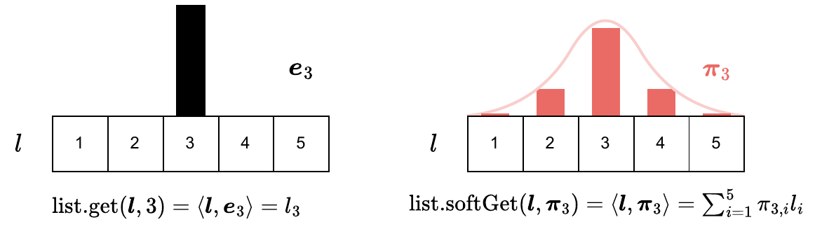
In order to be able to differentiate list.getw.r.t. indexing, a natural idea is to replace the integer index i∈[K] by a distribution πi∈△K, which we can interpret as a soft index. An integer index i∈[K] is then equivalent to a delta distributionπi∈{e1,…,eK}. We define the continuous relaxation list.softGet:LK(V)×△K→conv(V) as list.softGet(l,πi):=j=1∑Kπi,jlj=cond(πi,l1,…,lK)=EI∼Categorical(πi)[lI], where cond is studied in Section 5.7. In the particular case V=R, we obtain list.softGet(l,i)=⟨l,πi⟩. This is illustrated in Fig. 6.1.
The choice of the distribution πi=(πi,1,…,πi,K) encodes the importance of the elements (l1,…,lK)w.r.t. li. If we consider that the smaller ∣i−j∣ is, the more related li and lj are, then it makes sense to define a distribution centered around i (i.e., such that the mode of the distribution is achieved at i). For example, limiting ourselves to the neighborsli−1 and li+1 (i.e., a window of size 1), we can define the sparse distribution πi:=41⋅ei−1+21ei+41⋅ei+1∈△K. In this particular case, the continuous relaxation of the list.get function can then be expressed as a discrete convolution, list.softGet(l,πi)=(list.get(l,⋅)∗κ)(i)=j=−∞∑∞list.get(l,i−j)κ(j), where κ(−1):=41, κ(1):=41, κ(0):=21, and κ(j):=0 for j∈{−1,0,1}. Assuming V=RM, the computational complexity of list.softGet is O(M⋅∣supp(πi)∣).
Figure 6.1: The list.get(l,i) function is continuous and differentiable in l but not in i. Its relaxation list.softGet(l,πi) is differentiable in both l and πi. When V=R, list.softGet(l,πi) can be seen as taking the inner product between the list l and the probability distribution πi, instead of the delta distribution (canonical vector) ei.
Setting values
To differentiate w.r.t. indexing, we can define the continuous relaxation list.softSet:LK(V)×△K×V→LK(conv(V)) as [list.softSet(l,πi,v)]j:=E[list.set(l,I,v)]j=P(I=j)v+P(I=j)lj=πi,jv+(1−πi,j)lj, where j∈[K] and I∼Categorical(πi). Equivalently, we can write list.softSet(l,πi,v)=(πi,1v+(1−πi,1)l1,…,πi,Kv+(1−πi,K)lK)=(ifelse(πi,1,v,l1),…,ifelse(πi,K,v,lK)), where ifelse is studied in Section 5.6. Since ifelse(π,u1,u0)=EI∼Bernoulli(π)[uI], this relaxation amounts to using an element-wise expectation. As a result, the list output by list.softSet takes values in conv(V) instead of V. Note however that when V=RM, then conv(V)=RM as well.
Inserting values
To differentiate value insertion w.r.t. indexing, we can define the continuous relaxation list.softInsert:LK(V)×△K+1×V→LK+1(conv(V)) as [list.softInsert(l,πi,v)]j:=E[list.insert(l,I,v)]=P(I>j)lj+P(I=j)v+P(I<j)lj−1, where I∼Categorical(πi). The three necessary probabilities can easily be calculated for j∈[K+1] by P(I>j)P(I=j)P(I<j)={0∑k=j+1K+1πi,k if j=K+1 otherwise =πi,j={0∑k=1j−1πi,k if j=1 otherwise .
Multi-dimensional indexing
In multi-dimensional lists (arrays or tensors), each element li∈V of a list l∈LK1,…,KT(V) can now be indexed by a multivariate integer i=(i1,…,iT)∈[K1]×⋯×[KT], where T∈N is the number of axes of l. We can always flatten a multi-dimensional list into a uni-dimensional list by replacing the multi-dimensional index i∈[K1]×⋯×[KT] by a flat index i∈[K1…KT]. The converse operation, converting a flat uni-dimensional array into a multi-dimensional array, is also possible. Therefore, there is a bijection between [K] and [K1]×⋯×[KT] for K:=K1…KT.
This means that the previous discussion on soft indexing in the uni-dimensional setting readily applies to the multi-dimensional setting. All it takes is the ability to define a probability distribution πi∈△K1×⋯×KT. For example, when working with images, we can define a probability distribution putting probability mass only on the neighboring pixels of pixel i, a standard approach in image processing. Another simple approach is to use a product of axis-wise probability distributions.
6.2 Dictionaries
A dictionary (a.k.a. associative array or map) is an unordered list of key-value pairs, such that each possible key appears at most once in the list. We denote the set of keys by K and the set of values by V (both being potentially infinite). We can then define the set of dictionaries of size L from K to V by DL(K,V):=LL(K×V)=(K×V)L and one such dictionary by d:=((k1,v1),…,(kL,vL))∈DL(K,V).
6.2.1 Basic operations
Getting values
The goal of the dict.get function is to retrieve the value associated with a key, assuming that the dictionary contains this key. Formally, we define the dict.get:DL(K,V)×K→V∪{∞} function as dict.get(d,k):={vi∞ if ∃i∈[L] s.t. k=ki if k∈{k1,…,kL}. The function is continuous and differentiable in the dictionary d, but not in the key k. Equivalently, we can write the function as dict.get(d,k):=∑i=1Leq(k,ki)∑i=1Leq(k,ki)vi. The denominator encodes the fact that the function is undefined if no key in the dictionary d matches the key k. Assuming k∈{k1,…,kL} and V=RM, we can also write dict.get(d,k)=viwherei=j∈[L]argmax∥k−kj∥2, which shows that we can see dict.get as a nearest neighbor search.
Setting values
The goal of the dict.set function is to replace the value associated with an existing key. Formally, we define the dict.set:DL(K,V)×K×V→DL(K,V) function as (dict.set(d,k,v))i:={(ki,v)(ki,vi)ifki=kifki=k. The function leaves the dictionary unchanged if no key in the dictionary matches the input key k. The function is continuous and differentiable in d and v, but not in k.
Implementation
While we view dictionaries as lists of key-value pairs, in practice, a dictionary (a.k.a. associative array) is often implemented using a hash table or search trees. The hardware counterpart of a dictionary is called content-addressable memory (CAM), a.k.a. associative memory.
6.2.2 Continuous relaxation using kernel regression
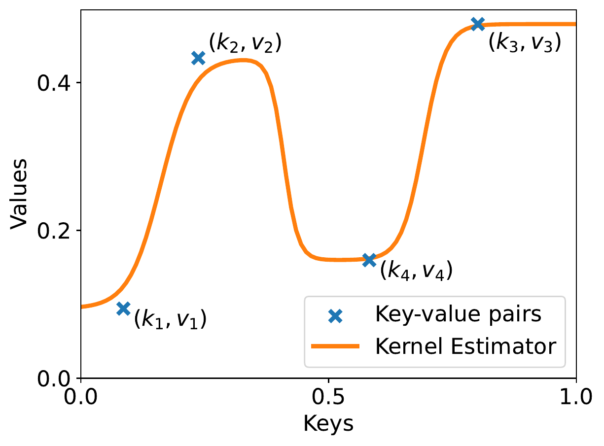
Figure 6.2: Given a set of key-value pairs (ki,vi)∈K×V defining a dictionary d, we can estimate a continuous mapping from K to V using Nadaraya–Watson kernel regression (here, illustrated with K=V=R). When keys are normalized to have unit norm, this recovers softargmax attention from Transformers.
A dictionary can be seen as a (potentially non-injective) function that associates a value v to each key k. To obtain a continuous relaxation of the operations associated to a dictionary, we can adopt a probabilistic perspective of the mapping from keys to values. We can view keys and values as two continuous random variables K and V. We can express the conditional PDF f(v∣k) of V∣K in terms of the joint PDF f(k,v) of (K,V) and the marginal PDF f(k) of K as f(v∣k)=f(k)f(k,v). Integrating, we obtain the conditional expectationE[V∣K=k]=∫Vf(v∣k)vdv=∫Vf(k)f(k,v)vdv. This is the Bayes predictor, in the sense that E[V∣K] is the minimizer of E[(h(K)−V)2] over the space of measurable functions h:K→V. Using a sample of L input-output pairs (ki,vi), corresponding to key-value pairs in our case, Nadaraya–Watson kernel regression estimates the joint PDF and the marginal PDF using kernel density estimation (KDE). Using a product of isotropic kernels κσ and ρσ for key-value pairs, we can define fσ(k,v):=L1i=1∑Lκσ(k−ki)ρσ(v−vi). The corresponding marginal distribution on the keys is then given as fσ(k):=∫Vfσ(k,v)dv=L1i=1∑Lκσ(k−ki)∫Vρσ(v−vi)dv=L1i=1∑Lκσ(k−ki). Replacing f with fσ, we obtain the following estimator of the conditional expectation E[V∣K=k]:=∫Vfσ(k)fσ(k,v)vdv=∫VL1∑i=1Lκσ(k−ki)L1∑i=1Lκσ(k−ki)ρσ(v−vi)vdv=∑i=1Lκσ(k−ki)∑i=1Lκσ(k−ki)∫Vρσ(v−vi)vdv=∑i=1Lκσ(k−ki)∑i=1Lκσ(k−ki)vi. In the above, we assumed that ρσ(v−vi)=pvi,σ(v), where pvi,σ(v) is the PDF of a distribution whose mean is vi, so that ∫Vρσ(v−vi)vdv=EV∼pvi,σ[V]=vi. Given a dictionary d=((k1,v1),…,(kL,vL)), we can therefore define the dict.softGet:DL(K,V)×K→conv(V) function as dict.softGet(d,k):=∑i=1Lκσ(k−ki)∑i=1Lκσ(k−ki)vi. This kernel regression perspective on dictionaries was previously pointed out by Zhang et al. (2021). It is illustrated in Fig. 6.2 with K=V=R.
6.2.3 Discrete probability distribution perspective
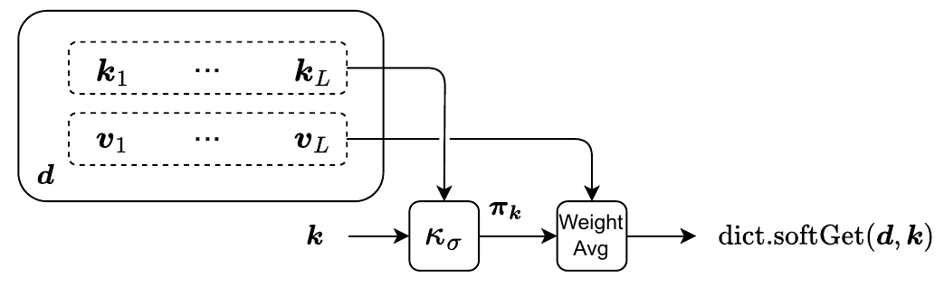
While the set of possible keys K is potentially infinite, the set of keys {k1,…,kL}⊂K associated with a particular dictionary d=((k1,v1),…,(kL,vL)) is finite. To a particular key k, we can therefore associate a discrete probability distribution πk=(πk,1,…,πk,L)∈△L over the keys (k1,…,kL) of d, defined by πk,i:=∑j=1Lκσ(k−kj)κσ(k−ki)∀i∈[L]. This distribution captures the affinity between the input key k and the keys (k1,…,kL) of dictionary d. As illustrated in Fig. 6.3, we obtain dict.softGet(d,k)=Ei∼Categorical(πk)[vi]=i=1∑Lπk,ivi. In the limit σ→0, we recover dict.get(d,k)=∑i=1Leq(k,ki)∑i=1Leq(k,ki)vi.
Figure 6.3: Computation graph of the dict.softGet function. We can use a kernel κσ to produce a discrete probability distribution πk=(πk,1,…,πk,L)∈△L, that captures the affinity between the dictionary keys (k1,…,kL) and the input key k. The dict.softGet function can then merely be seen as a convex combination (weighted average) of values (v1,…,vL) using the probability values (πk,1,…,πk,L) as weights.
While the dict.get function is using a mapping from keys k∈{k1,…,kL} to integer indices [L], the dict.softGet function is using a mapping from keys k∈{k1,…,kL} to distributions πk∈△L. This perspective allows us to reuse the soft functions we developed for lists in Section 6.1. For example, we can softly replace the value associated with key k by performing list.softSet(d,πk,(k,v)). Unlike dict.set, the function is differentiable w.r.t. the distribution πk.
6.2.4 Link with attention in Transformers
In the case when κσ is the Gaussian kernel, assuming that the keys are normalized to have unit norm (which is often the case in practical implementations (Dehghani et al., 2023; Schlag et al., 2021)), we obtain κσ(k−ki)=exp(−∥k−ki∥22/(2σ2))=exp(−(∥k∥22+∥ki∥22)/(2σ2))exp(⟨k,ki⟩/σ2)=exp(−1/σ2)exp(⟨k,ki⟩/σ2) so that πk,i=∑j=1Lκσ(k−kj)κσ(k−ki)=∑j=1Lexp(⟨k,kj⟩/σ2)exp(⟨k,ki⟩/σ2). We recognize the softargmax operator. Given a dictionary d=((k1,v1),…,(kL,vL)), we thus recover attention from Transformers (Vaswani et al., 2017) as dict.softGet(d,k)=i=1∑Lπk,ivi=i=1∑L∑j=1Lexp(⟨k,kj⟩/σ2)exp(⟨k,ki⟩/σ2)vi. Transformers can therefore be interpreted as relying on a differentiable dictionary mechanism. Besides Transformers, content-based memory addressing is also used in neural Turing machines (Graves et al., 2014).
6.3 Summary
Operations on lists are continuous and differentiable w.r.t. the list, but not w.r.t. the integer index. Similarly, operations on dictionaries are continuous and differentiable w.r.t. the dictionary, but not w.r.t. the input key.
Similarly to the way we handled the predicate in conditionals, we can replace the integer index (respectively the key) with a probability distribution over the indices (respectively the keys).
This allows us to obtain a probabilistic relaxation of operations on lists. In particular, the relaxation for list.get amounts to performing a convolution. The relaxation for dict.get amounts to computing a conditional expectation using kernel regression.
When using a Gaussian kernel with keys normalized to unit norm, we recover softargmax attention from Transformers.