Chapter 12Differentiating through integration
In this chapter, we study how to differentiate through integrals, with a focus on expectations and solutions of ordinary differential equations.
12.1 Differentiation under the integral sign
Given two Euclidean spaces and , and a function , we often want to differentiate an integral of the form Provided that we can swap integration and differentiation, we have The conditions enabling us to do so are best examined in the context of measure theory. We refer the reader to e.g. (Cohn, 2013) for a course on measure theory and Flanders (1973) for an in-depth study of the differentiation under the integral sign. Briefly, if , the following conditions are sufficient.
is measurable in both its arguments, and is integrable for almost all fixed,
is absolutely continuous for almost all , that is, there exists an integrable function such that ,
(which exists almost everywhere if is absolutely continuous), is locally integrable, that is, for any closed interval , the integral is finite.
Any differentiable function is absolutely continuous. However, the conditions also hold if is just absolutely continuous, that is, if is differentiable for almost all . This weaker assumption can be used to smooth out differentiable almost-everywhere functions, such as the ReLU, as we study in Section 14.4.
12.2 Differentiating through expectations
A special case of differentiating through integrals is differentiating through expectations. We can distinguish between two cases, depending on whether the parameters we wish to differentiate are involved in the distribution or in the function, whose expectation we compute.
12.2.1 Parameter-independent distributions
We first consider expectations of the form for a random variable , distributed according to a distribution , and a function . Importantly, the distribution is independent of the parameters . Under mild conditions recalled in Section 12.1, we can swap differentiation and integration to obtain Generally, the expectation cannot be computed in closed form. However, provided that we can sample from , we can define a Monte-Carlo estimator of the value and of the gradient
for i.i.d. samples from . These estimators are unbiased, meaning that and , and they converge to the true quantity as . This suggests a simple implementation in an autodiff framework of the approximation of :
Sample from .
Compute .
Compute the gradient by automatic differentiation.
Computing higher-order derivatives follows the same principle: to get an approximation of , we can simply compute by autodiff. As such, the implementation delineated above is akin to the “discretize-then-optimize” approach used to differentiate through the solution of an ODE (Section 12.6): we implement an approximation of the objective and simply call autodiff on it.
12.2.2 Parameter-dependent distributions
A more challenging case arises when the distribution depends on the parameters : where is a random variable, distributed according to a distribution parameterized by and where is, depending on the setting, potentially a blackbox function (i.e., we do not have access to its gradients). Typically, could be parameters we wish to estimate, or it could indirectly be generated by , where is a neural network with parameters we wish to estimate. The main difficulty in computing stems from the fact that are the parameters of the distribution . Estimating an expectation using Monte-Carlo estimation requires us to sample from . However, it is not clear how to differentiate w.r.t. if is involved in the sampling process.
Continuous case
When is a continuous set (that is, is a probability density function), we can rewrite as Provided that we can swap integration and differentiation (see Section 12.1), we then have Unfortunately, this integral is not an expectation and it could be intractable in general.
Discrete case
When is a discrete set (that is, is a probability mass function), we can rewrite as We then obtain Again, is not an expectation. We therefore cannot use Monte-Carlo estimation to estimate the gradient. Instead, we can compute it by brute force, i.e., by summing over all possible . However, this is clearly only computationally tractable if is small or if is designed to have sparse support, i.e., so that the set is small. Moreover, even if these conditions hold, summing over could be problematic if is expensive to compute. Therefore, exact gradients are seldom used in practice.
In Sections 12.3 and 12.4, we review the score function and pathwise gradient estimators, to (approximately) compute , allowing us to optimize (or using the chain rule) by gradient-based algorithms.
12.2.3 Application to expected loss functions
Differentiating through expectations is particularly useful when working with expected loss functions of the form where is some ground truth. Equivalently, we can set , where is a reward function. As we shall see, the score function estimator will support a discrete loss function , while the pathwise gradient estimator will require a differentiable loss function . Intuitively, will be low if assigns high probability to predictions with low loss value .
In the classification setting, where , is often chosen to be the Gibbs distribution, which is a categorical distribution induced by a softargmax where are logits produced by a neural network . More generally, in the structured prediction setting, where but , we often use the distribution where .
Given a distribution over , we then want to minimize the expected loss function, also known as risk, Typically, minimizing is done through some form of gradient descent, which requires us to be able to compute Computing therefore boils down to computing the gradient of , which is the gradient of an expectation.
12.2.4 Application to experimental design
In experimental design, we wish to minimize a function , which we assume costly to evaluate. As an example, evaluating could require us to run a scientific experiment with parameters . As another example, in hyperparameter optimization, evaluating would require us to run a learning algorithm with hyperparameters . Instead of solving the problem , we can lift the problem to probability distributions and solve , where . This requires the probability distribution to assign high probability to values that achieve small value. Solving this problem by stochastic gradient descent requires us to be able to compute estimates of . This can be done for instance with SFE explained in Section 12.3, which does not require gradients of , unlike implicit differentiation explained in Chapter 11. This approach also requires us to choose a distribution over . For continuous hyperparameters, a natural choice would be the normal distribution , setting . Once we have obtained by minimizing , we need a way to recover . This can be done for example by choosing the mode of the distribution, i.e., , or the mean of the distribution . Of course, in the case of the normal distribution, they coincide.
12.3 Score function estimators, REINFORCE
12.3.1 Scalar-valued functions
The key idea of the score function estimator (SFE), also known as REINFORCE, is to rewrite as an expectation. The estimator is based on the logarithmic derivative identity Using this identity, we obtain the following gradient estimator.
Proposition 12.1 (SFE for scalar-valued functions)
Given a family of distributions on , for , define where and . Then,
Proof
◻
The gradient of the log-PDF w.r.t. , , is known as the score function, hence the estimator name. SFE is suitable when two requirements are met: it is easy to sample from and the score function is available in closed form. Since the SFE gradient is an expectation, we can use Monte-Carlo estimation to compute an unbiased estimator of : where are sampled from .
Interestingly, the gradient of is not needed in this estimator. Therefore, there is no differentiability assumption about . This is why SFE is useful when is a discrete loss function or more generally a blackbox function.
Example 12.1 (SFE with a language model)
In a language model, the probability of a sentence is typically factored using the chain rule of probability (see Section 10.1) where is modeled using a transformer or RNN. Note that the probabilities are normalized by construction, so there is no need for an explicit normalization constant. Thanks to this factorization, it is easy to sample from using ancestral sampling (see Section 10.5.3) and the log-probability enjoys the simple expression This gradient is easy to compute, since the token-wise distributions are typically defined using a softargmax. We can therefore easily compute under using SFE. This is for instance useful to optimize an expected reward, in order to finetune or align a language model (Ziegler et al., 2019).
Another example when is available in closed form is in the context of reinforcement learning, where is a Markov Decision Process (MDP) and is called the policy. Applying the SFE leads to the (vanilla) policy gradient method (Sutton et al., 1999) and can then be used to compute the gradient of an expected cumulative reward. However, SFE is more problematic when used with the Gibbs distribution, due to the explicit normalization constant.
Example 12.2 (SFE with a Gibbs distribution)
The Gibbs distribution is parameterized, for , where we defined the log-partition function A typical parametrization is with the output of a network on a sample with parameters . We then have so that We therefore see that crucially depends on , the gradient of the log-partition. This gradient is available for some structured sets , see e.g. (Mensch and Blondel, 2018), but not in general.
As another example, we apply SFE in Section 14.4 to derive the gradient of perturbed functions.
Differentiating through both the distribution and the function
Suppose both the distribution and the function now depend on . When is scalar-valued and differentiable w.r.t. , we want to differentiate Using the product rule, we obtain
Differentiating through joint distributions
Suppose we now want to differentiate through The gradient is then given by which is easily seen by applying Proposition 12.1 on the joint distribution . The extension to more than two variables is straightforward.
12.3.2 Variance reduction
We discuss in this section various techniques for reducing the variance of estimators of , where .
Bias and variance
Recall the definition of in Eq. (12.1). SFE is an unbiased estimator, meaning that where the expectation is taken with respect to the samples drawn. Since the gradient is vector-valued, we need to define a scalar-valued notion of variance. We do so by using the squared Euclidean distance in the usual variance definition to define The variance naturally goes to zero as .
Baseline
SFE is known to suffer from high variance (Mohamed et al., 2020). This means that this estimator may require us to draw many samples from the distribution to work well in practice. One of the simplest variance reduction technique consists in shifting the function with a constant , called a baseline, to obtain The reason this is still a valid estimator of stems from for any valid distribution . The baseline is often set to the running average of past values of the function , though it is neither optimal nor does it guarantee to lower the variance (Mohamed et al., 2020).
REINFORCE leave-one-out (RLOO)
A simple way to reduce the variance is REINFORCE leave-one-out (RLOO) (Ahmadian et al., 2024; Kool et al., 2019). The key idea is to draw multiple independent samples from and for each sample , to use the remaining samples as a baseline. The RLOO gradient estimator is defined as This is an unbiased estimator, meaning that where the expectation is taken over . This comes from the independence of for , such that since by Bartlett’s first identity (12.2).
It can be checked that the estimator can equivalently be rewritten as This is slightly more convenient to implement, as we can use as a shared baseline across samples.
Control variates
Another general technique are control variates. Let us denote the expectation of a function under the distribution as Suppose that and its gradient are known in closed form. Then, for any , we clearly have and therefore Applying SFE, we then obtain Examples of function include a bound on or a second-order Taylor expansion of , assuming that these approximations are easier to integrate than (Mohamed et al., 2020).
12.3.3 Vector-valued functions
It is straightforward to extend the SFE to vector-valued functions.
Proposition 12.2 (SFE for vector-valued functions)
Given a family of distributions on , for , define where , . The JVP of at along is and the VJP of at along is The Jacobian of at can then be written as where denotes the outer product.
Proof
The VJP of at along amounts to computing the gradient of the scalar function The expression of the VJP follows by using the SFE on the scalar valued integrand . The JVP is obtained as the adjoint operator of the VJP and the Jacobian follows. ◻
Differentiating through both the distribution and the function
If now influences both the distribution and the function, then, we obtain
12.3.4 Second derivatives
Using the previous subsection with , we easily obtain an estimator of the Hessian.
Proposition 12.3 (SFE for the Hessian)
Let us define the scalar-valued function . Then,
This can also be derived using the second-order log-derivative so that
Link with the Bartlett identities
The Bartlett identities are expressions relating the moments of the score function (gradient of the log-likelihood function). Using Proposition 12.1 with and , we obtain which is known as Bartlett’s first identity. Similarly, using Proposition 12.3, we obtain which is known as Bartlett’s second identity.
12.3.5 Autodiff-friendly implementation
So far, we derived expressions of score function estimators for first and second derivatives. From a user perspective, instead of manually implementing these expressions, it would be more convenient if we could just call autodiff on some function and recover the correct expressions of the score function estimators. This can be achieved using the so-called magicbox operator (Foerster et al., 2018). This operator is defined as where is the stop gradient operator.
During the evaluation of a program, the stop gradient operator acts as the identity. During automatic differentiation, that is, during forward or reverse mode autodiff, this operator stops any flow of derivatives. In other words, its Jacobian is zero on any inputs despite evaluating as the identity. Such an operator does not exist mathematically, but it can be defined in an autodiff framework using custom derivation rules. Evaluations and derivatives of programs making intervene are then to be understood first in terms of the autodiff framework and its custom rules.
Coming back to the magicbox operator, its evaluation and its derivatives in an autodiff framework are then for any The “magic” happens when we compose the magicbox operator with another function. Consider a (twice) differentiable function . We then have Let be a sample from and let us define . Then, correctly recovering the expressions for the first derivative in Proposition 12.1 and for the second derivative in Proposition 12.3. Let us define the functions We then correctly obtain for all The key benefit is that is compatible with autodiff frameworks, while is not. In practice, we can draw samples (without differentiating through the sampling) and define By Monte-Carlo estimation, we then have where the expectation is taken over .
12.4 Path gradient estimators, reparametrization trick
As we saw previously, the main difficulty in computing gradients of expectations arises when the parameters play a role in the distribution being sampled. The key idea of path gradient estimators (PGE), also known as reparametrization trick, is to rewrite the expectation in such a way that the parameters are moved from the distribution to the function, using a change of variable.
12.4.1 Location-scale transforms
The canonical example of path gradient estimator is differentiating through the expectation where is a differentiable function. If we let , it is easy to check that . We can therefore write The key advantage is that we can now easily compute the derivatives by mere application of the chain rule, since the parameters and are moved from the distribution to the function: The change of variable is called a location-scale transform. Such a transformation exists, not only for the normal distribution, but for location-scale family distributions, i.e., distributions parametrized by a location parameter and a scale parameter , such that is distributed according to a distribution in the same family as is distributed. Besides the normal distribution, examples of location-scale family distributions include the Cauchy distribution, the uniform distribution, the logistic distribution, the Laplace distribution, and Student’s -distribution.
We can easily relate the cumulative distribution function (CDF) and the probability density function (PDF) of to that of , and vice-versa.
Proposition 12.4 (CDF and PDF of location-scale family distributions)
Let and . If , then
Proof
We have and we obtain by differentiating . ◻
12.4.2 Differentiable transforms
We can generalize the idea of path gradient estimator (PGE) to any change of variable where is a differentiable transformation. For example, if we gather and as , we can write the location-scale transform as We can derive the path gradient estimator for any such differentiable transformation .
Proposition 12.5 (Path gradient estimator)
Let us define where and is differentiable. Suppose there is a differentiable transformation such that if (where does not depend on ) and , then . Then, we have where . This implies
The path gradient estimator (a.k.a. reparametrization trick) gives an unbiased estimator of . It has however two key disadvantages. First, it assumes that is differentiable (almost everywhere), which may not always be the case. Second, it assumes that is well-defined on , not on , which could be problematic for some discrete loss functions, such as the zero-one loss function or ranking loss functions.
As an example of differentiable transform, in machine learning, we can sample Gaussian noise and make it go through a neural network with parameters to generate an image . In statistics, many distributions are related to each other through differentiable transforms, as we recall below.
Example 12.3 (Some differentiable transforms in statistics)
We give below a non-exhaustive list of differentiable transform examples.
If , then .
If , then .
If (i.i.d.), then .
If for , then .
12.4.3 Inverse transforms
The inverse transform method can be used for sampling from a probability distribution, given access to its associated quantile function. Recall that the cumulative distribution function (CDF) associated with a random variable is the function defined by The quantile function is then a function such that for . Assuming is continuous and strictly increasing, we have that is the inverse CDF, In the general case of CDF functions that are not strictly increasing, the quantile function is usually defined as Given access to the quantile function associated with a distribution , inverse transform sampling allows us to sample from by first drawing a sample from the uniform distribution and then making this sample go through the quantile function.
Proposition 12.6 (Inverse transform sampling)
Suppose ,
where is a distribution with quantile function . If , then .
Proof
If , then by definition of , . If , then by definition of , , so and since a CDF is always non-decreasing, . Hence, we have, , so The CDFs of and coincide, hence they have the same distribution. ◻
If the quantile function is differentiable, we can therefore use it as a transformation within the reparametrization trick. Indeed, if , where is a distribution with parameter and quantile function , then we have and therefore, by the reparametrization trick (Proposition 12.5),
Example 12.4 (Examples of quantile functions)
If
, the CDF of is for and therefore the quantile function is . If , the CDF is and the quantile function is , where . This therefore defines an alternative transformation to the location-scale transformation in Eq. (12.4).
Note that, in the above example, the error function and its inverse do not enjoy analytical expressions but autodiff packages usually provide numerical routines to compute them and differentiate through them. Nonetheless, one caveat of the inverse transform is that it indeed requires access to (approximations of) the quantile function and its derivatives, which may be difficult for complicated distributions.
12.4.4 Pushforward operators
Pushforward distributions
We saw so far that the reparametrization trick is based on using a change of variables in order to differentiate an expectation w.r.t. the parameters of the distribution. In this section, we further formalize that approach using pushforward distributions.
Definition 12.1 (Pushforward distribution)
Suppose , where is a distribution over . Given a continuous map , the pushforward distribution of through is the distribution according to which is distributed, i.e., .
Although not explicit in the above, the transformation can depend on some learnable parameters, for example if is a neural network. Intuitively, the pushforward distribution is obtained by moving the position of all the points in the support of . We give a few examples below.
Inverse transform sampling studied in Section 12.4.3 can be seen as performing the pushforward of the uniform distribution through , where is the quantile function.
The Gumbel trick studied in Section 14.5 can be seen as the pushforward of Gumbel noise through (a discontinuous function).
Gumbel noise can itself be obtained by pushing forward the uniform distribution through (Remark 14.4).
In a generative modeling setting, as we mentioned previously, we use the pushforward of Gaussian noise through a parametrized transformation called a generator, typically a neural network.
It is possible to define distributions over (sparse) probability vectors by sampling then projecting (Farinhas et al., 2021).
A crucial aspect of the pushforward distribution is that it can be implicitly defined, meaning that we do not necessarily need to know the explicit form of the associated PDF. In fact, it is easy to sample from , provided that it is easy to sample from : Hence the usefulness of the pushforward distribution in generative modeling. Furthermore, if has associated PDF , we can compute the expectation of a function according to as even though we do not know the explicit form of the PDF of .
Pushforward measures
More generally, we can define the notion of pushforward, in the language of measures. Denote the set of measures on a set . A measure , that has a density , can be integrated against a function as A measure is called a probability measure if it is positive and satisfies . See Peyré and Cuturi (2019, 2) for a concise introduction.
Definition 12.2 (Pushforward operator and measure)
Given a continuous map and some measure , the pushforward measure is such that for all continuous functions Equivalently, for any measurable set , we have where .
Importantly, the pushforward operator preserves positivity and mass, therefore if is a probability measure, then so is . The pushforward of a probability measure therefore defines a pushforward distribution (since a distribution can be parametrized by a probability measure).
12.4.5 Change-of-variables theorem
We saw that a pushforward distribution associated with a variable is implicitly defined through a transform and can be easily sampled from as long as it is easy to sample . However, in some applications (e.g., density estimation), we may want to know the PDF associated with . Assuming the transform is invertible, we have and therefore for , we have Using the change-of-variables theorem from multivariate calculus, assuming is available, we can give an explicit formula for the PDF of the pushforward distribution, see e.g. (Schwartz, 1954; Taylor, 2002).
Proposition 12.7 (PDF of the pushforward distribution)
Suppose
, where is a distribution over , with PDF . Given a diffeomorphism (i.e., an invertible and differentiable map), the pushforward distribution of through is the distribution such that and its PDF is where is the Jacobian of .
Using this formula, we obtain Using the inverse function theorem (Theorem 11.7), we then have under the assumption that is continuously differentiable and has invertible Jacobian . Normalizing flows are parametrized transformations designed such that and its Jacobian are easy to compute; see e.g. Kobyzev et al. (2019; Papamakarios et al., 2021) for a review.
12.5 Stochastic programs
A stochastic program is a program that involves some form of randomness. In a stochastic program, the final output, as well as intermediate variables, may therefore be random variables. In other words, a stochastic program induces a probability distribution over program outputs, as well as over execution trajectories.
12.5.1 Stochastic computation graphs
A stochastic program can be represented by a stochastic computation graph as originally introduced by Schulman et al. (2015). Departing from that work, our exposition explicitly supports two types of intermediate operations: sampling from a conditional distribution or evaluating a function. These operations can produce either deterministic variables or random variables.
Function and distribution nodes
Formally, we define a stochastic computation graph as a directed acyclic graph , where , is the set of function nodes and is the set of distribution nodes. Similarly to computation graphs reviewed in Section 4.1.3, we number the nodes as . Node corresponds to the input , which we assume to be deterministic. It is the variable with respect to which we wish to differentiate. Node corresponds to the program output , which we assume to be a random variable. A node can either be a function node with an associated function or a distribution node , with associated conditional distribution . A stochastic program has at least one distribution node, the source of randomness. Otherwise, it is a deterministic program. As for computation graphs, the set of edges is used to represent dependencies between nodes. We denote the parents of node by .
Deterministic and random variables
We distinguish between two types of intermediate variables: deterministic variables and random variables . Therefore, a distribution or a function may receive both types of variables as conditioning or input. It is then convenient to split as , where we defined the deterministic parents and the random parents . Therefore, are the deterministic parent variables and are the random parent variables, of node .
Executing a stochastic program
We assume that nodes are in topological order (if this is not the case, we need to perform a topological sort). Given parent variables and , a node produces an output as follows.
If (distribution node), the output is Note that technically is the distribution of conditioned on its parents, not the distribution of . Therefore, we should in principle write . We avoid this notation for conciseness and for symmetry with function nodes.
Contrary to a function node, a distribution node can have no parents. That is, if , it is possible that . A good example would be a parameter-free noise distribution.
If (function node), the output is in general and in the special case , the output is
Unless the associated conditional distribution is a delta distribution, that puts all the probability mass on a single point, the output of a distribution node is necessarily a random variable . For function nodes , the output of the function is a random variable if at least one of the parents of produces a random variable. Otherwise, if all parents of produce deterministic variables, the output of is a deterministic variable .
The entire procedure is summarized in Algorithm 12.1. We emphasize that is a random variable. Therefore, a stochastic program (implicitly) induces a distribution over , and also over intermediate random variables . Executing the stochastic program allows us to draw samples from that distribution.
Algorithm 12.1: Executing a stochastic program
Nodes: in topological order, where node is either a function or a conditional distribution
Input: input
for do
Retrieve
if then ▷ Distribution node
else if then ▷ Function node
if then
▷ Output is a R.V.
else if then
▷ Output is deterministic
Output:
Special cases
If all nodes are function nodes, we recover computation graphs, reviewed in Section 4.1.3. If all nodes are distribution nodes, we recover Bayesian networks, reviewed in Section 10.5.
12.5.2 Examples
We now present several examples that illustrate our formalism. We use the legend below in the following illustrations.

Example 1 (SFE estimator):
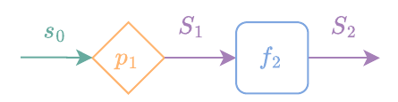
Example 2 (Pathwise estimator):
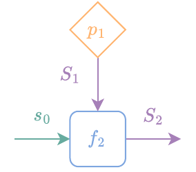
Example 3 (SFE estimator + chain rule):

Example 4:
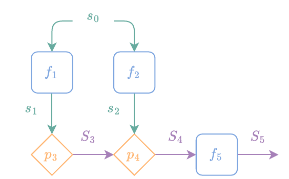
As can be seen, the gradient expressions can quickly become quite complicated, demonstrating the merits of automatic differentiation in stochastic computation graphs.
12.5.3 Unbiased gradient estimators
The output of a stochastic program is a random variable It implicitly defines a probability distribution such that . Executing the stochastic program once gives us an i.i.d. sample from .
Since derivatives are defined for deterministic variables, we need a way to convert a random variable to a deterministic variable. One way to do so is to consider the expected value (another way would be the mode) where the expectation is over or equivalently over the intermediate random variables for (the distribution nodes). We then wish to compute the gradient or more generally the Jacobian of .
If all nodes in the stochastic computation graph are function nodes, we can estimate the gradient of using the pathwise estimator a.k.a. reparametrization trick (Section 12.4). This is the approach taken by Kingma and Welling (2013) and Rezende et al. (2014).
If all nodes in the stochastic computation graph are distribution nodes, we can use the SFE estimator (Section 12.3). Schulman et al. (2015) propose a surrogate loss so that using autodiff on that loss produces an unbiased gradient of the expectation, using the SFE estimator. Foerster et al. (2018) extend the approach to support high-order differentiation. Krieken et al. (2021) further extend the approach by supporting different estimators per node, as well as control variates.
Converting distribution nodes into function nodes and vice-versa
Our formalism uses two types of nodes: distribution nodes with associated conditional distribution and function nodes with associated function . It is often possible to convert between node types.
Converting a distribution node into a function node is exactly the reparametrization trick studied in Section 12.4. We can use transformations such as the location-scale transform or the inverse transform.
Converting a function node into a distribution node can be done using the change-of-variables theorem, studied in Section 12.4.5, on a pushforward distribution.
Because the pathwise estimator has lower variance than SFE, this is the method of choice when the functions are available. The conversion from distribution node to function node and vice-versa is illustrated in Fig. 12.1.
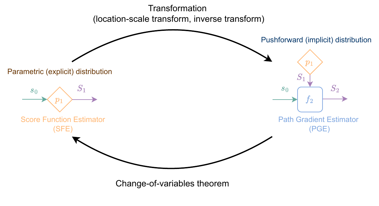
Figure 12.1: It is sometimes possible to convert a distribution node to a function node and vice-versa using a suitable transformation.
12.5.4 Local vs. global expectations
A stochastic computation graph can be seen as a stochastic process, a collection of random variables , indexed by , the position in the topological order. However, random variables are incompatible with autodiff. Replacing random variables by their expectation can be seen as a way to make them compatible with autodiff. Two strategies are then possible.
As we saw in the previous section, a strategy is to consider the expectation of the last output . This strategy corresponds to a global smoothing. The two major advantages are that i) we do not need to assume that is well-defined on and ii) this induces a probability distribution over program executions. This is for instance useful to compute the variance of the program. The gradient of the program’s expected value can be estimated by the reparametrization trick or by the SFE, depending on the type of nodes used.
A second strategy is to replace an intermediate random variable , for , by its expectation . This strategy corresponds to a local smoothing. A potential drawback of this approach is that belongs to , the convex hull of . Therefore, the function in which is fed must be well-defined on , which may not always be the case. In the case of control flows, another disadvantage is computational. We saw in Section 5.6 and Section 5.7 that using a soft comparison operator within a conditional statement induces a distribution on a binary or categorical random variable, corresponding to the branch to be selected. A conditional statement can then be locally smoothed out by replacing the random variable by its expectation i.e., a convex combination of all the branches. This means that, unless the distribution has sparse support, all branches must be evaluated.
12.6 Differential equations
12.6.1 Parameterized differential equations
From residual networks to neural ODEs
Starting from , residual networks, reviewed in Section 4.6, iterate for A residual network can be seen as parameterizing incremental discrete-time input changes (hence the name “residual”) Chen et al. (2018) proposed to parameterize continuous-time (instantaneous) changes instead. They considered the evolution of the inputs in continuous time driven by a function parameterized by , starting from . Formally, the evolution is the solution of the ordinary differential equation (ODE) Here, is the vector of derivatives of as defined in Remark 2.4, and denotes a final time for the trajectory. The output of such a neural ODE (Chen et al., 2018) is then . Alternatively, the output can be seen as the solution of an integration problem Differential equations like Eq. (12.5) arise in many contexts beyond neural ODEs, ranging from modeling physical systems to pandemics (Braun and Golubitsky, 1983). Moreover, the differential equation presented in Eq. (12.5) is just an example of an ordinary differential equation, while controlled differential equations or stochastic differential equations can also be considered.
Existence of a solution
First and foremost, the question is whether is well-defined. Fortunately, the answer is positive under mild conditions, as shown by Picard-Lindelöf’s theorem recalled below (Butcher, 2016, Theorem 16).
Theorem 12.1 (Existence and uniqueness of ODE solutions)
If is continuous in its first variable and Lipschitz-continuous in its second variable, then there exists a unique differentiable map satisfying for some given .
For time-independent linear functions , the integral in Eq. (12.6) can be computed in closed form as where is the matrix exponential. Hence, the output can be expressed as a simple function of the parameters ( in this case). However, generally, we do not have access to such analytical solutions, and, just as for solving optimization problems in Chapter 11, we need to resort to some iterative algorithms.
Integration methods
To numerically solve an ODE, we can use integration methods, whose goal is to build a sequence that approximates the solution at times . The simplest integration method is the explicit Euler method, which approximates the solutions between times and as for a time-step The resulting integration scheme consists in computing starting from , for , Assimilating with , we find that residual networks are essentially the discretization of a neural ODE by an explicit Euler method; more precisely, a non-autonomous neural ODE, see e.g. (Davis et al., 2020).
Euler’s forward method is only one integration method among many. To cite a few, there are implicit Euler methods, semi-implicit methods, Runge-Kutta methods, linear multistep methods, etc. See, e.g., Gautschi (2011) for a detailed review. The quality of an integration method is measured by its consistency and its stability (Gautschi, 2011). These concepts naturally influence the development of evaluation and differentiation techniques for ODEs. We briefly summarize them below.
Given a fixed time interval and points, an integration method is consistent of order if as and therefore . The higher the order , the fewer points we need to reach an approximation error on the points considered. The term is reminiscent of the error encountered in finite differences (Chapter 7) and is called the truncation error.
The (absolute) stability of a method is defined by the set of time-steps such that the integration method can integrate for some without blowing up as .
12.6.2 Continuous adjoint method
Since different parameters induce different trajectories associated with in Eq. (12.5), we may want to select one of these trajectories by minimizing some criterion. For example, we may consider selecting by minimizing a loss on the final point of the trajectory, where To solve such problems, we need to access gradients of composed with through VJPs of the solution of the ODE. The VJPs can actually be characterized as solutions of an ODE themselves thanks to the continuous time adjoint method (Pontryagin, 1985), presented below, and whose proof is postponed to Section 12.6.6.
Proposition 12.8 (Continuous-time adjoint method)
Consider a function , continuous in its first variable, Lipschitz-continuous and continuously differentiable in its second variable. Assume that exists for any , and is also continuous in its first variable, Lipschitz-continuous in its second variable. Denote the solution of the ODE and the final state of the ODE at time .
Then, the function is differentiable, and for an output direction , its VJP along is given by for and for solving the adjoint (backward) ODE In particular, the gradient for a differentiable loss is obtained by solving the adjoint ODE with .
Example 12.5 (Fitting data through the solution of an ODE)
As an illustrative example, we can consider optimizing the parameters of an ODE to fit some data points. Namely, we may seek a continuous time solution of a modified Lotka Volterra ODE for , that fits some observations . The optimization problem then consists of and requires backpropagating through the solution of the ODE w.r.t. its candidate parameters . Fig. 12.2 illustrates such a problem with varying candidate parameters.
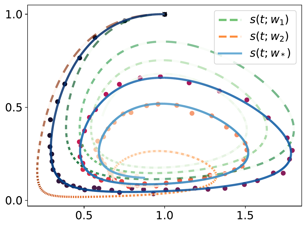
Figure 12.2: Finding the optimal parameters of an ODE to fit some observed data. The dots represent the trajectories of a dynamical system observed at regular times (time is represented here by a gradient color, the lighter the color, the larger the time). Each line represents the solution of an ODE given by some hyperparameters . The objective is to find the hyperparameters of the ODE such that its solution fits the data points. Green and orange lines fail to do so while the blue line fits the data. To compute such parameters , we need to backpropagate through the solution of the ODE.
12.6.3 Gradients via the continuous adjoint method
Proposition 12.8 gives a formal definition of the gradient. However, just as computing the mapping itself, computing its VJP or the gradient of requires solving an integration problem. Note that the integration of in Proposition 12.8 requires also values of . Therefore, we need to integrate both and . Such an approach is generally referred to as optimize-then-discretize because we first formulate the gradient in continuous time (the “optimize part”) and then discretize the resulting ODE.
Simple discretization scheme
A first approach consists in defining a backward discretization scheme that can approximate backward in time. Namely, by defining , and , the derivative of is given by . The functions are solutions of a standard ODE The above ODE can then be solved by any integration method. Note, however, that it requires first computing and by an integration method. The overall computation of the gradient using an explicit Euler method to solve forward and backward ODEs is summarized in Algorithm 12.2.
Algorithm 12.2: Gradient computation via continuous adjoint method with Euler explicit discretization
Functions: ,
Inputs: input , parameters , number of discretization steps .
Set discretization step , denote .
Set
for do ▷ Forward discretization
Compute .
Compute .
Initialize , ,
for do ▷ Backward discretization
Compute
Compute
Compute
Output:
Algorithm 12.2 naturally looks like the reverse mode of autodiff for a residual neural network with shared weights. A striking difference is that the intermediate computations are not kept in memory and, instead, new variables are computed along the backward ODE. One may believe that by switching to continuous time, we solved the memory issues encountered in reverse-mode autodiff. Unfortunately, this comes at the cost of numerical stability. As we use a discretization scheme to recompute the intermediate states backward in time through in Algorithm 12.2, we accumulate some truncation errors.
To understand the issue here, consider applying Algorithm 12.2 repeatedly on the same parameters but using instead of each time. In the continuous realm, . But after discretization, does not match . Therefore, by applying Algorithm 12.2 with , we would not get the same output even if in continuous time we naturally should have. This phenomenon is illustrated in Fig. 12.3. It intuitively shows why Algorithm 12.2 induces some noise in the estimation of the gradient.
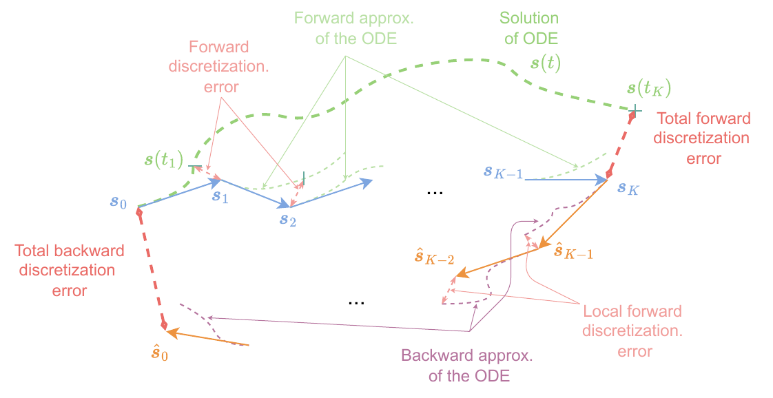
Figure 12.3: Forward and backward discretizations when using the continuous adjoint method.
Multiple shooting scheme
An alternative approach consists in integrating both the forward and backward ODEs jointly. Namely, we may solve an ODE with boundary values by means of a multiple shooting method or a collocation method (Stoer et al., 1980). This approach still requires to be approximated first.
12.6.4 Gradients via reverse-mode on discretization
A simpler approach consists in replacing the objective in Eq. (12.7) by its version discretized using some numerical method, such as an Euler forward discretization scheme. That is, we seek to solve with and some discretization step. Gradients of the objective can be computed by automatic differentiation. That approach is often referred to as discretize-then-optimize. At first glance, this approach may suffer from very high memory requirements. Indeed, to get an accurate solution of the ODE, a numerical integration method may require to be very large. Since a naive implementation of reverse-mode automatic differentiation has a memory that scales linearly with , computing the gradient by a discretize-then-optimize method could be prohibitive. However, the memory requirements may easily be amortized using checkpointing, as explained in Section 8.5; see also (Gholaminejad et al., 2019).
As for the optimize-then-discretize method, we still accumulate some truncation errors in the forward discretization process. This discretization error occurs when computing the gradient in reverse-mode too. The discretize-then-optimize method can be seen as computing gradients of a surrogate objective. For that objective, the gradients are correct and well-defined. However, they may not match the gradients of the true ODE formulation.
To compare the discretize-then-optimize and optimize-then-discretize approaches, Gholaminejad et al. (2019) compared their performance on an ODE whose solution can be computed analytically by selecting to be linear in . The authors observed that discretize-then-optimize generally outperformed optimize-then-discretize. A middle ground can actually be found by using reversible differentiation schemes.
12.6.5 Reversible discretization schemes
Our exposition of the optimize-then-discretize or discretize-then-optimize approaches used a simple Euler explicit discretization scheme. However, for both approaches, we could have used other discretization schemes instead, such as reversible discretization schemes.
A reversible discretization scheme is a discretization scheme such that we have access to a closed-form formula for the inverse of its discretization step. Formally, a discretization method builds an approximation of the solution of an ODE on an interval by computing for where is some fixed discretization step, is the time step (typically ), is the approximation of , and is some additional context variable used by the discretization method to build the iterates. An explicit Euler method does not have a context, but just as an optimization method may update some internal states, a discretization method can update some context variable. The discretization scheme in Eq. (12.8) is a forward discretization scheme as we took a positive discretization step. By taking a negative discretization step, we obtain the corresponding backward discretization scheme, for , A discretization method is reversible if we have access to to recompute the inputs of the discretization step from its outputs, A reversible discretization method is symmetric if the backward discretization scheme is exactly the inverse of the forward discretization scheme, i.e., The explicit Euler method is clearly not symmetric and a priori not reversible, unless we can solve for , the equation .
Leapfrog method
The (asynchronous) leapfrog method (Mutze, 2013; Zhuang et al., 2021) on the other hand is an example of symmetric reversible discretization method. For a constant discretization step , given and a function , it computes One can verify that we indeed have .
By using a reversible symmetric discretization scheme in the optimize-then-discretize approach, we ensure that, at the end of the backward discretization pass, we recover exactly the original input. Therefore, by repeating forward and backward discretization schemes we always get the same gradient, which was not the case for an Euler explicit scheme.
By using a reversible discretization scheme in the discretize-then-optimize method, we address the memory issues of reverse mode autodiff. As explained in Section 8.6, we can recompute intermediate values during the backward pass rather than storing them.
Momentum residual networks
In the leapfrog method, the additional variables may actually be interpreted as velocities of a system whose acceleration is driven by the given function, that is, . Such an interpretation suggests alternatives to the usual neural ODE paradigm. For instance, momentum neural networks (Sander et al., 2021b), can be interpreted as the discretization of a second-order ordinary differential equation, which is naturally amenable to reversible differentiation schemes with a low memory footprint.
12.6.6 Proof of the continuous adjoint method
In the following, we denote the solution of the ODE at time given the input and the parameters . We focus here on the formulation of the VJP. The proof relies on the existence of partial derivatives of , which we do not cover here and refer to, e.g., Pontryagin (1985) for a complete proof of such facts given the assumptions.
We use the ODE constraint to introduce adjoint variables, this time in the form of a continuously differentiable function . For any such function , we have using Leibniz notations such as . The VJPs then decompose as Here the second derivative terms correspond to second derivatives of . Since the Hessian is symmetric (Schwarz’s theorem presented in Proposition 2.10), we can swap the derivatives in and or . Then, to express the gradient uniquely in terms of first derivatives of , we use an integration by parts to have for example Since , we have . The VJP w.r.t. can then be written as By choosing to satisfy the adjoint ODE the expression of the VJP simplifies as For the VJP w.r.t. , we can proceed similarly. Using an integration by parts, we have, this time, since . Choosing the same curve satisfying the adjoint ODE we get The existence of a curve solution of the backward ODE can easily be shown from Picard Lindelöf’s theorem and the assumptions.
12.7 Summary
We studied how to differentiate integrals, with a focus on expectations and solutions of a differential equation.
For differentiating through expectations, we studied two main methods: the score function estimator (SFE, a.k.a. REINFORCE) and the path gradient estimator (PGE, a.k.a. reparametrization trick).
The SFE is suitable when it is easy to sample from the distribution and its log-PDF is explicitly available. It is an unbiased estimator, but is known to suffer from high variance.
The PGE is suitable for pushforward distributions, distributions that are implicitly defined through a transformation, or a sequence of them. These distributions can be easily sampled from, by injecting a source of randomness (such as noise) through the transformations. An unbiased, low-variance estimator of the gradient of their expectation is easily obtained, provided that we can interchange integration and differentiation.
If we have an explicit distribution, we can sometimes convert it to an implicit distribution, thanks to the location-scale transformation or the inverse transformation.
Conversely, if we have an implicit distribution, we can convert it to an explicit distribution using the change-of-variables theorem. However, this formula requires computing the determinant of an inverse Jacobian, and is computationally expensive in general. Normalizing flows use invertible transformations so that the inverse Jacobian is cheap to compute, by design.
Stochastic computation graphs can use a mix of explicit and implicit distributions at each node.
For differentiating through the solution of a differential equation, two approaches can be considered.
We can express the gradient as the solution of a differential equation thanks to the continuous adjoint method. We may then discretize backwards in time the differential equation that the gradient satisfies. This is the optimize-then-discretize approach.
We can also first discretize the problem in such a way that the gradient can simply be computed by reverse mode auto-diff, applied on the discretization steps. This is the discretize-then-optimize approach. The optimize-then-discretize approach has no memory cost, but discrepancies between the forward and backward discretization passes often lead to numerical errors. The discretize-then-optimize approach introduces no such discrepancies but may come at a large memory cost.
Reversible discretization schemes can circumvent the memory cost, as they enable the recomputation of intermediate discretization steps backwards in time.