Chapter 10Inference in graphical models as differentiation

A graphical model specifies how random variables depend on each other and therefore determines how their joint probability distribution factorizes. In this chapter, we review key concepts in graphical models and how they relate to differentiation, drawing in the process analogies with computation chains and computation graphs.

10.1 Chain rule of probability

The chain rule of probability is a fundamental law in probability theory for computing the joint probability of events. In the case of only two events $A_1$ and $A_2$, it reduces to the product rule $$\PP(A_1 \cap A_2) = \PP(A_2 | A_1) \PP(A_1).$$ For two discrete random variables $S_1$ and $S_2$, using the events $A_1 \coloneqq \{S_1 = \s_1\}$ and $A_2 \coloneqq \{S_2 = \s_2\}$, the product rule becomes $$\PP(S_1= \s_1, S_2= \s_2) = \PP(S_2=\s_2 | S_1=\s_1) \PP(S_1=\s_1).$$ More generally, using the product rule, we have for $K$ events $$\PP\left(A_1 \cap \ldots \cap A_K\right) = \PP\left(A_K \mid A_1 \cap \ldots \cap A_{K-1}\right) \PP\left(A_1 \cap \ldots \cap A_{K-1}\right).$$ Applying the product rule one more time, we have $$\PP\left(A_1 \cap \ldots \cap A_{K-1}\right) = \PP\left(A_{K-1} \mid A_1 \cap \ldots \cap A_{K-2}\right) \PP\left(A_1 \cap \ldots \cap A_{K-2}\right).$$ Repeating the process recursively, we arrive at the chain rule of probability $$\begin{align*} \PP\left(A_1 \cap \ldots \cap A_K\right) &= \prod_{j=1}^K \PP(A_j \mid A_1 \cap \dots \cap A_{j-1})\\ &= \prod_{j=1}^K \PP\left(A_j \,\Bigg|\, \bigcap_{i=1}^{j-1} A_i\right). \end{align*}$$ For $K$ discrete random variables $S_j$, using the events $A_j \coloneqq \{S_j = \s_j \}$, the chain rule of probability becomes $$\PP\left(S_1 = \s_1, \ldots,S_K = \s_K\right) = \prod_{j=1}^K \mathbb P(S_j = \s_j \mid S_1 = \s_1, \dots, S_{j-1}=\s_{j-1}).$$ Importantly, this factorization holds without any independence assumption on the variables $S_1,\dots,S_K$. In other words, the space of probability distributions specified by the joint probability on the left-hand side, and the space of probability distributions specified by the product of conditional probabilities on the right-hand side, are the same. We can further simplify the factorization if we make additional conditional independence assumptions.

10.2 Conditional independence

We know that if two events $A$ and $B$ are independent, then $$\PP(A|B) = \PP(A).$$ Similarly, if two random variables $S_1$ and $S_2$ are independent, then $$\PP(S_2=\s_2|S_1=\s_1) = \PP(S_2=\s_2).$$ More generally, if we work with $K$ variables $S_1, \dots, S_K$, some variables may depend on each other, while others may not. To simplify the notation, given a set $\cC$, we define the shorthands $$\begin{align*} S_\cC &\coloneqq (S_i \colon i \in \cC) \\ \s_\cC &\coloneqq (\s_i \colon i \in \cC). \end{align*}$$ We say that a variable $S_j$ is independent of $S_\cD$ conditioned on $S_\cC$, with $\cC \cap \cD = \emptyset$, if for any $\s_j, \s_{\cC}, \s_{\cD}$ $$\PP(S_j = \s_j \mid S_\cC = \s_\cC, S_\cD = \s_\cD) = \PP(S_j = \s_j \mid S_\cC = \s_\cC).$$

10.3 Inference problems

10.3.1 Joint probability distributions

We consider a collection of $K$ variables $\s \coloneqq (\s_1, \dots, \s_K)$, potentially ordered or unordered. Each $\s$ belongs to the Cartesian product $\cS \coloneqq \cS_1 \times \dots \times \cS_K$. Throughout this chapter, we assume that the sets $\cS_k$ are discrete for concreteness, with $\cS_k \coloneqq \{\v_1, \dots, \v_{M_k}\}$. Note that because $\cS_k$ is discrete, we can always identify it with $\{1,\dots,M_k\}$. A graphical model specifies a joint probability distribution $$\begin{align*} \PP(S = \s) &= \PP(S_1=\s_1,\dots,S_K=\s_K) \\ &= p(\s) \\ &= p(\s_1,\dots,\s_K), \end{align*}$$ where $p$ is the probability mass function of the joint probability distribution. Summing over the Cartesian product of all possible configurations, we obtain $$\sum_{\s \in \cS} p(\s) = \sum_{\s_1,\dots,\s_K \in \cS} p(\s_1,\dots,\s_K) = 1.$$ As we shall see, the graph of a graphical model encodes the dependencies between the variables $(S_1,\dots,S_K)$ and therefore how their joint distribution factorizes. Given access to a joint probability distribution, there are several inference problems one typically needs to solve.

10.3.2 Likelihood

A simple task is to compute the likelihood of some observations $\s = (\s_1,\dots,\s_K)$, $$\PP(S_1 = \s_1, \dots, S_K = \s_K) = p(\s_1, \dots, \s_K).$$ It is also common to compute the log-likelihood, $$\log \PP(S_1 = \s_1, \dots, S_K = \s_K) = \log p(\s_1, \dots, \s_K).$$

10.3.3 Maximum a-posteriori inference

Another common task is to compute the most likely configuration, $$\argmax_{\s_1 \in \cS_1, \dots, \s_K \in \cS_K} p(\s_1,\dots,\s_K).$$ This is the mode of the joint probability distribution. This is also known as maximum a-posteriori (MAP) inference in the literature (Wainwright and Jordan, 2008).

10.3.4 Marginal inference

The operation of marginalization consists in summing (or integrating) over all possible values of a given variable in a joint probability distribution. This allows us to compute the marginal probability of the remaining variables. For instance, we may want to marginalize all variables but $S_k=\s_k$. To do so, we define the Cartesian product $$\begin{align*} \cC_k(\s_k) \coloneqq \underbrace{\cS_1 \times \dots \times \cS_{k-1}}_{\cA_{k-1}} \times \{\s_k\} \times \underbrace{\cS_{k+1} \times \dots \times \cS_K}_{\cB_{k+1}}. \tag{10.1}\end{align*}$$ Summing over all variables but $S_k$, we obtain the marginal probability of $S_k=\s_k$ as $$\begin{align*} \PP(S_k = \s_k) &= \sum_{\s_1,\dots,\s_K \in \cC_k(\s_k)} p(\s_1,\dots,\s_K) \\ &= \sum_{\s_1,\dots,\s_{k-1} \in \cA_{k-1}} \sum_{\s_{k+1},\dots,\s_K \in \cB_{k+1}} p(\s_1,\dots,\s_K). \end{align*}$$ Defining similarly $$\begin{align*} \cC_{k,l}(\s_k,\s_l) \coloneqq \cS_1 \times \dots \times \{\s_k\} \times \dots \times \{\s_l\} \times \dots \times \cS_K, \end{align*}$$ we obtain $$\begin{align*} \PP(S_k = \s_k, S_l=\s_l) = \sum_{\s_1,\dots,\s_K \in \cC_{k,l}(\s_k,\s_l)} p(\s_1,\dots,\s_K). \end{align*}$$ In particular, we may want to compute the marginal probability of two consecutive variables, $\PP(S_{k-1} = \s_{k-1}, S_k=\s_k)$.

10.3.5 Expectation, convex hull, marginal polytope

Another common operation is to compute the expectation of $\phi(S)$ under a distribution $p$. It is defined by $$\begin{align*} \muv \coloneqq \EE_{S \sim p}[\phi(S)] = \sum_{\s \in \cS} p(\s) \phi(\s) \in \cM. \end{align*}$$ For the expectation under $p_\thetav$, we write $$\begin{align*} \mu(\thetav) \coloneqq \EE_{S \sim p_\thetav}[\phi(S)] = \sum_{\s \in \cS} p_\thetav(\s) \phi(\s) \in \cM. \end{align*}$$ In exponential family distributions (Section 3.4), the function $\phi$ is called a statistic. It decomposes as $$\begin{align*} \phi(\s) \coloneqq (\phi_\cC(\s_\cC))_{\cC \in C}, \end{align*}$$ where $\cC \subseteq [K]$. Intuitively, $\phi(\s)$ can be thought of as an encoding or embedding of $\s$ (a potentially discrete object such as a sequence of integers) in a vector space. Under this decomposition, we can also compute $$\muv_\cC \coloneqq \EE_S[\phi_\cC(S_\cC)] = \sum_{\s \in \cS} p(\s) \phi_\cC(\s_\cC).$$

Convex hull

The mean $\muv$ belongs to the convex hull of $\phi(\cS) \coloneqq \{\phi(\s) \colon \s \in \cS\}$, $$\cM \coloneqq \conv(\phi(\cS)) \coloneqq \left\{ \sum_{\s \in \cS} p(\s) \phi(\s) \colon p \in \cP(\cS) \right\},$$ where $\cP(\cS)$ is the set of all possible probability distributions over $\cS$. In other words, $\cM$ is the set of all possible convex combinations of $\phi(\s)$ for $\s \in \cS$. The vertices of $\cM$ are all the $\s \in \cS$.

Case of binary encodings: the marginal polytope

In the special case of a discrete set $\cS_k = \{\v_1,\dots,\v_M\}$ and of a binary encoding (indicator function) $\phi(\s)$, the set $\cM$ is called the marginal polytope (Wainwright and Jordan, 2008), because each point $\muv \in \cM$ contains marginal probabilities. To see why, consider the unary potential $$[\phi(\s)]_{k,i} = [\phi_k(\s_k)]_{i} = \II(\s_k = \v_i) \tag{10.2}$$ where $\II(p) \coloneqq 1$ if $p$ is true, $0$ otherwise. We then obtain the marginal probability of $S_k=\v_i$, $$\begin{align*} [\muv]_{k,i} &= \EE_S[\phi(S)_{k,i}] \\ &= \EE_{S_k}[\phi_k(S_k)_i] \\ &= \EE_{S_k}[\II(S_k=\v_i)] \\ &= \sum_{\s_k \in \cS_k} \PP(S_k=\s_k)\II(\s_k=\v_i) \\ &= \PP(S_k = \v_i). \end{align*}$$ Likewise, consider the pairwise potential $$[\phi(\s)]_{k,l,i,j} = [\phi_{k,l}(\s_k, \s_l)]_{i,j} = \II(\s_k = \v_i, \s_l=\v_j) . \tag{10.3}$$ We then obtain the marginal probability of $S_k=\v_i$ and $S_l=\v_j$, $$\begin{align*} [\muv]_{k,l,i,j} &= \EE_S[\phi(S)_{k,l,i,j}] \\ &= \EE_{S_k,S_l}[\phi_{k,l}(S_k,S_l)_{i,j}] \\ &= \EE_{S_k,S_l}[\II(S_k=\v_i,S_l=\v_j)] \\ &= \sum_{\s_k \in \cS_k} \sum_{\s_l \in \cS_l} \PP(S_k=\s_k,S_l=\s_l) \II(\s_k=\v_i,\s_l=\v_j) \\ &= \PP(S_k=\v_i, S_l = \v_j). \end{align*}$$ We can do the same with higher-order potential functions.

10.3.6 Complexity of brute force

Apart from computing the likelihood, which is trivial, computing the marginal, mode and expectation by brute force takes $O(\prod_{k=1}^K |\cS_k|)$ time. In particular, if $|\cS_k| = M ~\forall k \in [K]$, brute force takes $O(M^K)$ time.

10.4 Markov chains

In this section, we briefly review Markov chains. Our notation is chosen to emphasize the analogies with computation chains.

10.4.1 The Markov property

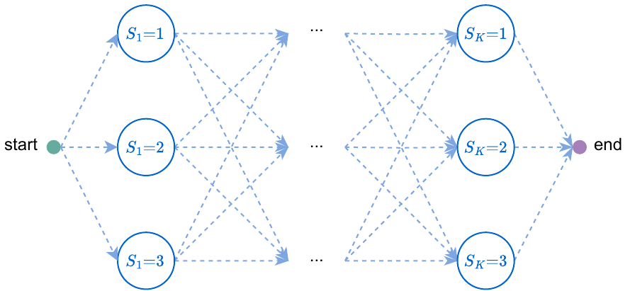
When random variables are organized sequentially as $S_1,\dots,S_K$, a simple example of conditional independence is when each variable $S_k \in \cS_k$ only depends on the previous variable $S_{k-1} \in \cS_{k-1}$, that is, $$\begin{align*} \PP(S_k=\s_k \mid S_{k-1}=\s_{k-1}, \dots, S_1=\s_1) &= \PP(S_k=\s_k \mid S_{k-1}=\s_{k-1}) \\ &\coloneqq p_k(\s_k \mid \s_{k-1}). \end{align*}$$ A probability distribution satisfying the above is said to satisfy the Markov property, and is called a Markov chain. A computation chain is specified by the functions $f_k$, that take $\s_{k-1}$ as input and output $\s_k$. In analogy, a Markov chain is specified by the conditional probability distributions $p_k$ of $S_k$ given $S_{k-1}$. We can then define the generative process $$\begin{align*} S_0 &\coloneqq \s_0 \\ S_1 &\sim p_1(\cdot \mid S_0) \\ S_2 &\sim p_2(\cdot \mid S_1) \\ &\vdots \\ S_K &\sim p_K(\cdot \mid S_{K-1}). \end{align*}$$ Strictly speaking, we should write $S_k \mid S_{k-1} \sim p_k(\cdot \mid S_{k-1})$. We choose our notation both for conciseness and for analogy with computation chains. Furthermore, to simplify the notation, we assume without loss of generality that $S_0$ is deterministic (if this is not the case, we can always move $S_0$ to $S_1$ and add a dummy variable as $S_0$). That is, $\PP(S_0 = \s_0) = p_0(\s_0) \coloneqq 1$ and $\cS_0 \coloneqq \{\s_0\}$. This amounts to setting the initial distribution of $S_1$ as $$\PP(S_1 = \s_1) \coloneqq \PP(S_0 = \s_0) \PP(S_1 = \s_1 | S_0 = \s_0) = \PP(S_1 = \s_1 | S_0 = \s_0).$$ We can then compute the joint probability of the Markov chain by $$\begin{align*} \PP(S_1=\s_1,\dots,S_K=\s_K) &= p(\s_1,\dots,\s_K) \\ &= \prod_{k=1}^K \PP(S_k = \s_k \mid S_{k-1} = \s_{k-1}) \\ &= \prod_{k=1}^K p_k(\s_k \mid \s_{k-1}), \end{align*}$$ where we left the dependence on $\s_0$ implicit, since $p_0(\s_0) = 1$. A Markov chain with $\cS_k = \{1,2,3\}$ is illustrated in Fig. 10.1. A chain defines a totally ordered set $\{1, \dots, K\}$, since two nodes in the graph are necessarily linked to each other by a path.

10.4.2 Time-homogeneous Markov chains

A time-homogeneous discrete-time Markov chain corresponds to the case when the distribution of $S_k$ given $S_{k-1}$ is the same regardless of $k$: $$p_1 = \dots = p_K = p.$$ The finite-space case corresponds to when each $S_k \in \cS$ can take a finite set of values $\cS = \{\v_1,\dots,\v_M\}$ and $$\PP(S_k=\v_j \mid S_{k-1} = \v_i) = p(\v_j|\v_i) = \pi_{i,j},$$ where $\pi_{i,j} \in [0,1]$ is the transition probability from $\v_i$ to $\v_j$. Because the set $\cS = \{\v_1,\dots,\v_M\}$ is discrete, we can always identify it with $\{1,\dots,M\}$. That is, we can instead write $$\PP(S_k=j \mid S_{k-1} = i) = p(j|i) = \pi_{i,j}.$$

10.4.3 Higher-order Markov chains

More generally, a $n^{\text{th}}$-order Markov chain may depend, not only on the last variable, but on the last $n$ variables, $$\begin{align*} &\PP(S_k=\s_k \mid S_{k-1}=\s_{k-1}, \dots, S_1=\s_1) \\ = &\PP(S_k=\s_k \mid S_{k-1}=\s_{k-1}, \dots, S_{k-n}=\s_{k-n}) \\ = &p_k(\s_k|\s_{k-1},\dots,\s_{k-n}). \end{align*}$$ Autoregressive models such as Transformers (Section 4.8) can be seen as specifying a higher-order Markov chain, with a context window of size $n$. The larger context makes exact inference using dynamic programming computationally intractable. This is why practitioners use beam search or ancestral sampling (Section 10.5.3) instead.

10.5 Bayesian networks

In this section, we briefly review Bayesian networks. Our notation is chosen to emphasize the analogies with computation graphs.

10.5.1 Expressing variable dependencies using DAGs

Markov chains and more generally higher-order Markov chains are a special case of Bayesian network. Similarly to computation graphs reviewed in Section 8.3, variable dependencies can be expressed using a directed acyclic graph (DAG) $\cG = (\cV, \cE)$, where the vertices $\cV = \{1, \dots, K\}$ represent variables and edges $\cE$ represent variable dependencies. The set $\{i_1, \dots, i_{n_k}\} = \parent(k) \subseteq \cV$, where $n_k \coloneqq |\parent(k)|$, indicates the variables $S_{i_1},\dots,S_{i_{n_k}}$ that $S_k$ depends on. This defines a partially ordered set (poset). For notational simplicity, we again assume without loss of generality that $S_0$ is deterministic. A computation graph is specified by functions $f_1,\dots,f_K$ in topological order. In analogy, a Bayesian network is specified by conditional probability distributions $p_k$ of $S_k$ given $S_{\parent(k)}$. We can then define the generative process $$\begin{align*} S_0 &\coloneqq \s_0 \\ S_1 &\sim p_1(\cdot \mid S_0) \\ S_2 &\sim p_2(\cdot \mid S_{\parent(2)}) \\ &\vdots \\ S_K &\sim p_K(\cdot \mid S_{\parent(K)}). \end{align*}$$ Using the chain rule of probability and variable independencies expressed by the DAG, the joint probability distribution is then (assuming a topological order for $S_0,S_1,\dots, S_K$) $$\begin{align*} \PP(S = \s) &\coloneqq \PP(S_1=\s_1, \dots, S_K=\s_K) \\ &= \prod_{k=1}^K \PP(S_k = \s_k| S_{\parent(k)} = \s_{\parent(k)}) \\ &\coloneqq \prod_{k=1}^K p_k(\s_k|\s_{\parent(k)}). \end{align*}$$ This representation is well suited to express causal relationships between random variables.

10.5.2 Parameterizing Bayesian networks

In a Bayesian framework, observed data, latent variables, parameters and noise variables are all treated as random variables. If the conditional distribution $p_k$ associated to node $k$ depends on some parameters, they can be provided to $p_k$ as conditioning, using parent nodes.

A Bayesian network is specified by the conditional distributions $p_k$. Therefore, unlike computation graphs, there is no notion of function $f_k$ in a Bayesian network. However, the root nodes of the Bayesian network can be the output of a neural network. For instance, autoregressive models, such as RNNs or Transformers, specify the conditional probability distribution of a token given past tokens, and the chain rule of probability is used to obtain a probability distribution over entire sequences.

10.5.3 Ancestral sampling

A major advantage of Bayesian networks is that, provided that each conditional distribution $p_k$ is normalized, the joint distribution of $S = (S_1, \dots, S_K)$ is automatically normalized. This means that we can very easily draw i.i.d. samples from the joint distribution, by following the generative process: we follow the topological order $k= 1, \dots, K$ and on iteration $k$ we draw a value $\s_k \sim p_k(\cdot|\s_{\parent(k)})$ conditioned on the previous values $\s_{\parent(k)}$. This is known as ancestral sampling.

10.6 Markov random fields

10.6.1 Expressing factors using undirected graphs

A Markov random field (MRF), a.k.a. undirected graphical model, specifies a distribution that factorizes as $$\PP(S=\s) = p(\s) \coloneqq \frac{1}{Z} \prod_{\cC \in C} \psi_\cC(\s_\cC),$$ where $C$ is the set of maximal cliques of $\cG$, that is, subsets of $\cV$ that are fully connected, $Z$ is a normalization constant defined by $$Z \coloneqq \sum_{\s \in \cS} \prod_{\cC \in C} \psi_\cC(\s_\cC),$$ and $\psi_\cC \colon \cS_\cC \to \RR_+$ is a potential function (a.k.a. compatibility function), with $\cS_\cC \coloneqq (\cS_j)_{j \in \cC}$. According to the Hammersley-Clifford theorem, an MRF can be equivalently defined in terms of Markov properties; we refer the interested reader to Wainwright and Jordan (2008). For the sake of this chapter, the definition above is sufficient for our purposes.

10.6.2 MRFs as exponential family distributions

Let us define the potential functions $$\psi_\cC(\s_\cC; \thetav_\cC) \coloneqq \exp(\langle \thetav_\cC, \phi_\cC(\s_\cC) \rangle)$$ for some sufficient statistic function $\phi_\cC \colon \cS_\cC \to \Theta_\cC$ and parameters $\thetav_\cC \in \Theta_\cC$. Then, $$\begin{align*} p_\thetav(\s) &\coloneqq \frac{1}{Z(\thetav)} \prod_{\cC \in C} \psi_\cC(\s_\cC; \thetav_\cC) \\ &= \frac{1}{Z(\thetav)} \prod_{\cC \in C} \exp(\langle \thetav_\cC, \phi_\cC(\s_\cC) \rangle) \\ &= \frac{1}{Z(\thetav)} \exp\left(\sum_{\cC \in C} \langle \thetav_\cC, \phi_\cC(\s_\cC) \rangle\right) \\ &= \frac{1}{Z(\thetav)} \exp\left(\langle \thetav, \phi(\s) \rangle\right) \\ &= \exp\left(\langle \thetav, \phi(\s) \rangle - A(\thetav)\right) \end{align*}$$ where $$\begin{align*} \phi(\s) &\coloneqq (\phi_\cC(\s_\cC))_{\cC \in C} \\ \thetav &\coloneqq (\thetav_\cC)_{\cC \in C} \\ Z(\thetav) &\coloneqq \sum_{\s \in \cS} \prod_{\cC \in C} \psi_\cC(\s_\cC; \thetav_\cC) \\ &= \sum_{\s \in \cS} \exp\left(\langle \thetav, \phi(\s) \rangle\right) \\ A(\thetav) &\coloneqq \log Z(\thetav). \end{align*}$$ Therefore, for this choice of potential functions, we can view an MRF as an exponential family distribution (Section 3.4) with natural parameters $\thetav$, sufficient statistic $\phi$ and log-partition function $A(\thetav)$.

10.6.3 Conditional random fields

Conditional random fields (Lafferty et al., 2001; Sutton et al., 2012) are a special case of Markov random field, in which a conditioning variable is explicitly incorporated. For example, when the goal is to predict a variable $\y$ conditioned on a variable $\x$, CRFs are defined as $$\PP(Y=\y \mid X = \x) = p(\y \mid \x) = \frac{1}{Z(\x)} \prod_{\cC \in C} \psi_\cC(\y_\cC, \x).$$ Note that the potential functions $\psi_\cC$ are allowed to depend on the whole $\x$, as $\x$ is just a conditioning variable.

10.6.4 Sampling

Contrary to Bayesian networks, MRFs require an explicit normalization constant $Z$. As a result, sampling from a distribution represented by a general MRF is usually more involved than for Bayesian networks. A commonly-used technique is Gibbs sampling.

10.7 Inference on chains

In this section, we review how to perform marginal inference and maximum a-posteriori inference on joint distributions of the form $$p(\s_1,\dots,\s_K) = \frac{1}{Z} \prod_{k=1}^K \psi_k(\s_{k-1},\s_k),$$ where $$Z \coloneqq \sum_{\s \in \cS} \prod_{k=1}^K \psi_k(\s_{k-1},\s_k)$$ and where we used $\psi_k$ as a shorthand for $\psi_{k-1,k}$, since $k-1$ and $k$ are consecutive. As explained in Example 10.2, this also includes Markov chains by setting $$\psi_k(\s_{k-1},\s_k) \coloneqq p_k(\s_k \mid \s_{k-1}),$$ in which case $Z=1$.

10.7.1 The forward-backward algorithm

The key idea of the forward-backward algorithm is to use the distributivity of multiplication over addition to write $$Z = \sum_{\s_1 \in \cS_1} \psi_1(\s_0, \s_1) \sum_{\s_2 \in \cS_2} \psi_2(\s_1, \s_2) \dots \sum_{\s_K \in \cS_K} \psi_K(\s_{K-1}, \s_K).$$ We can compute these sums recursively, either forward or backward. Recalling the definitions of $\cA_{k-1}$ and $\cB_{k+1}$ in Eq. (10.1), we define the summations up to and down to $k$, $$\begin{align*} \alpha_k(\s_k) &\coloneqq \sum_{\s_1,\dots,\s_{k-1} \in \cA_{k-1}} \prod_{j=1}^k \psi_j(\s_{j-1}, \s_j) \\ &= \sum_{\s_{k-1} \in \cS_{k-1}} \psi_k(\s_{k-1}, \s_k) \dots \sum_{\s_1 \in \cS_1} \psi_2(\s_1,\s_2) \psi_1(\s_0,\s_1) \\ \beta_k(\s_k) &\coloneqq \sum_{\s_{k+1},\dots,\s_K \in \cB_{k+1}} \prod_{j=k+1}^K \psi_j(\s_{j-1}, \s_j) \\ &= \sum_{\s_{k+1} \in \cS_{k+1}} \psi_{k+1}(\s_k,\s_{k+1}) \dots \sum_{\s_K \in \cS_K} \psi_K(\s_{K-1},\s_K). \end{align*}$$ We can compute the two quantities by recursing forward and backward $$\begin{align*} \alpha_k(\s_k) &= \sum_{\s_{k-1} \in \cS_{k-1}} \psi_k(\s_{k-1},\s_k) \alpha_{k-1}(\s_{k-1}) \\ \beta_k(\s_k) &= \sum_{\s_{k+1} \in \cS_{k+1}} \psi_{k+1}(\s_k,\s_{k+1}) \beta_{k+1}(\s_{k+1}) \end{align*}$$ where we defined the initializations $$\begin{align*} \alpha_1(\s_1) &\coloneqq \psi_1(\s_0, \s_1) \quad \forall \s_1 \in \cS_1 \\ \beta_K(\s_K) &\coloneqq 1 \quad \forall \s_K \in \cS_K. \end{align*}$$ The normalization term can then be computed by $$\begin{align*} Z = \sum_{\s_K \in \cS_K} \alpha_K(\s_K) \beta_K(\s_K) = \sum_{\s_1 \in \cS_1} \alpha_1(\s_1) \beta_1(\s_1) \end{align*}$$ and the marginal probabilities by $$\begin{align*} \PP(S_k = \s_k) &= \frac{1}{Z} \alpha_k(\s_k) \beta_k(\s_k)\\ \PP(S_{k-1}=\s_{k-1}, S_k=\s_k) &= \frac{1}{Z} \alpha_{k-1}(\s_{k-1}) \psi_k(\s_{k-1}, \s_k) \beta_k(\s_k). \end{align*}$$ We can also compute the conditional probabilities by $$\begin{align*} \PP(S_k=\s_k \mid S_{k-1}=\s_{k-1}) &= \frac{\PP(S_{k-1}=\s_{k-1}, S_k=\s_k)}{\PP(S_{k-1}=\s_{k-1})} \\ &= \frac{\alpha_{k-1}(\s_{k-1}) \psi_k(\s_{k-1}, \s_k) \beta_k(\s_k)}{ \alpha_{k-1}(\s_{k-1}) \beta_{k-1}(\s_{k-1})} \\ &= \frac{\psi_k(\s_{k-1}, \s_k) \beta_k(\s_k)}{ \beta_{k-1}(\s_{k-1})}. \end{align*}$$ In practice, the two recursions are often implemented in the log-domain for numerical stability, $$\begin{align*} \log \alpha_k(\s_k) &= \log \sum_{\s_{k-1} \in \cS_{k-1}} \exp(\log \psi_k(\s_{k-1},\s_k) + \log \alpha_{k-1}(\s_{k-1})) \\ \log \beta_k(\s_k) &= \log \sum_{\s_{k+1} \in \cS_{k+1}} \exp(\log \psi_{k+1}(\s_k,\s_{k+1}) + \log \beta_{k+1}(\s_{k+1})). \end{align*}$$ We recognize the log-sum-exp operator, which can be implemented in a numerically stable way (Section 4.4.2). The overall dynamic programming procedure, a.k.a. forward-backward algorithm (Baum and Petrie, 1966; Rabiner, 1989), is summarized in Algorithm 10.1. We notice that the forward and backward passes are actually independent of each other, and can therefore be performed in parallel.