Chapter 9Second-order automatic differentiation

We review in this chapter how to perform automatic differentiation for second-order derivatives.

9.1 Hessian-vector products

We consider in this section a function $f \colon \cE \to \RR$ . Similarly to the Jacobian, for most purposes, we do not need access to the full Hessian but rather to the Hessian-vector product (HVP) $\nabla^2 f(\w) [\v]$ at $\w \in \cE$ , in a direction $\v \in \cE$ , as defined in Definition 2.19. The latter can be computed in four different ways, depending on how we combine the two main modes of autodiff.

9.1.1 Four possible methods

An HVP can be computed in four different ways.

Reverse on reverse: The Hessian can be seen as the transposed Jacobian of the gradient, hence the HVP can be computed as the VJP of the gradient, $\nabla^2 f(\w)[\v] = \partial (\nabla f)(\w)^*[\v].$
Forward on reverse: Owing to its symmetry (see Proposition 2.10), the Hessian can also be seen as the Jacobian of the gradient, hence the HVP can be computed as the JVP of the gradient, $\nabla^2 f(\w)[\v] = \partial (\nabla f)(\w)[\v].$
Reverse on forward: Recall that for any function $g \colon \cE \to \cE$ , the VJP can equivalently be defined as the gradient along an output direction $\v \in \cE$ , that is, $\partial g(\w)^*[\v] = \nabla \langle g, \v\rangle(\w),$ where we recall the shorthand $\langle g, \v \rangle(\w) \coloneqq \langle \v, g(\w) \rangle$ , so that $\langle g, \v \rangle$ is a function of $\w$ . In our case, we can therefore rewrite the reverse-on-reverse approach as $\partial (\nabla f)(\w)^*[\v] = \nabla \langle \nabla f, \v\rangle(\w).$ We know that $\langle \nabla f, \v\rangle(\w) = \langle \nabla f(\w), \v\rangle = \partial f(\w)[\v]$ is the JVP of $f$ at $\w$ along $\v$ . Therefore, we can also compute the HVP as the gradient of the JVP of $f$ at $\w$ along $\v$ , $\nabla^2 f(\w)[\v] = \nabla (\partial f(\cdot)[\v])(\w),$ where we use the notation $(\partial f(\cdot)[\v])(\w) \coloneqq \partial f(\w)[\v]$ to insist on the fact that it is a function of $\w$ .
Forward on forward: Finally, we can use the definition of the HVP in Definition 2.19 as a vector of second partial derivatives along $\v$ and each canonical direction. That is, assuming $\cE = \RR^P$ , we can compute the JVP of the JVP $P$ times: $\nabla^2 f(\w)[\v] = (\partial^2 f(\w)[\v, \e_i])_{i=1}^P.$

The four different ways of computing the HVP are summarized in Table 9.1.

Method	Computation
Reverse on reverse (VJP of gradient)	$\partial (\nabla f)(\w)^*[\v]$
Forward on reverse (JVP of gradient)	$\partial (\nabla f)(\w)[\v]$
Reverse on forward (gradient of JVP)	$\nabla (\partial f(\cdot)[\v])(\w)$
Forward on forward (JVPs of JVPs)	$(\partial^2 f(\w)[\v, \e_i])_{i=1}^P$

Table 9.1: Four different ways of computing the HVP $\nabla^2 f(\w)[\v]$ .

9.1.2 Complexity

To get a sense of the computational and memory complexity of the four approaches, we consider a chain of functions $f \coloneqq f_K \circ \dots \circ f_1$ as done in Section 8.1. To simplify our analysis, we assume $f_k \colon \RR^P \to \RR^P$ for $k \in \{1, \dots, K-1\}$ and $f_K \colon \RR^P \to \RR$ .

The computation graph of the reverse mode is illustrated in Fig. 9.1. While $f = f_K \circ \dots \circ f_1$ would be represented by a simple chain, the computational graph of $\nabla f$ is no longer a chain: it is a DAG. This is due to the computations of $\partial f_k(\s_{k-1})^*[\r_k]$ , where both $\s_{k-1}$ and $\r_k$ depend on $\s_0$ .

We illustrate the computation graphs of reverse-on-reverse and forward-on-reverse in Fig. 9.2 and Fig. 9.3 respectively. By applying reverse mode on reverse mode, at each fan-in operation $\s_{k-1}, \r_k \mapsto \partial f_k(\s_{k-1})^*[\r_k]$ , the reverse mode on $\nabla f$ branches out into two paths that are later merged by a sum. By applying forward mode on top of reverse mode, the flow of computations simply follows that of $\nabla f$ .

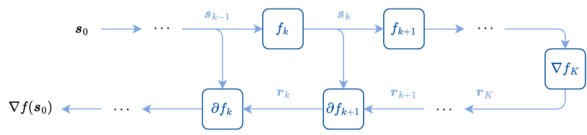
Figure 9.1: Computation graph corresponding to reverse mode autodiff for evaluating the gradient of $f=f_K \circ \ldots \circ f_1$ . While $f$ is a simple chain, $\nabla f$ is a DAG.

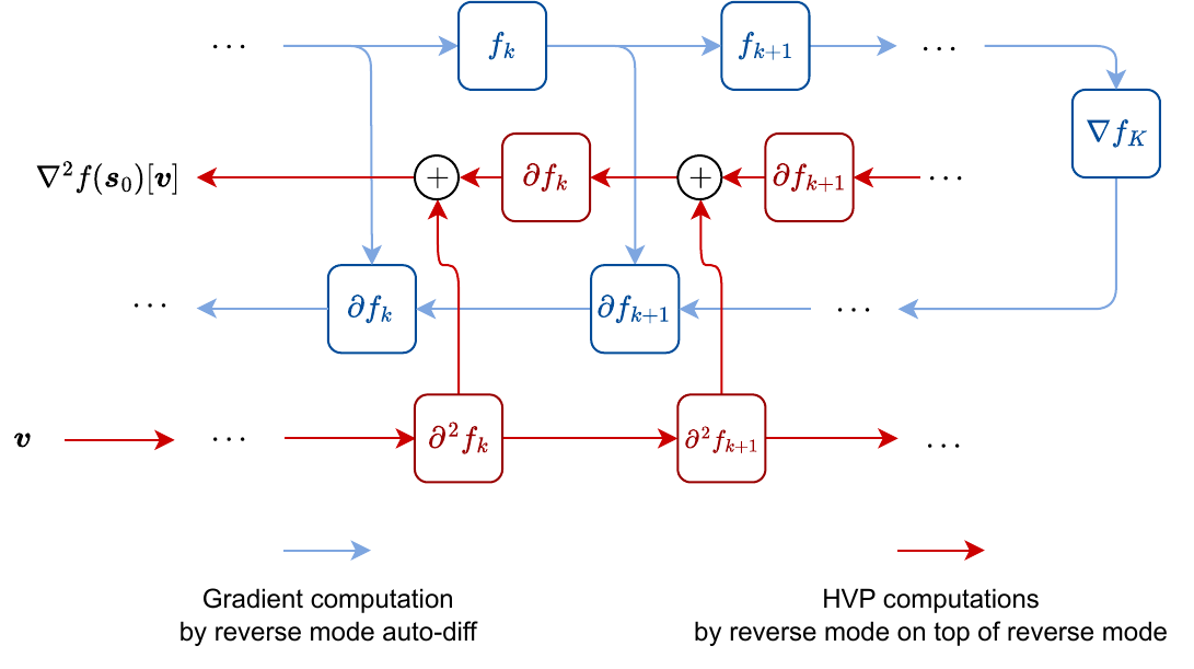
Figure 9.2: Computation graph for computing the HVP $\nabla^2 f(\w)[\v]$ by using reverse mode on top of reverse mode. As the computation graph of $\nabla f$ induces fan-in operations $\s_{k-1}, \r_k \mapsto \partial f_k(\s_{k-1})^*[\r_k]$ , the reverse mode applied on $\nabla f$ induces branching of the computations at each such node.

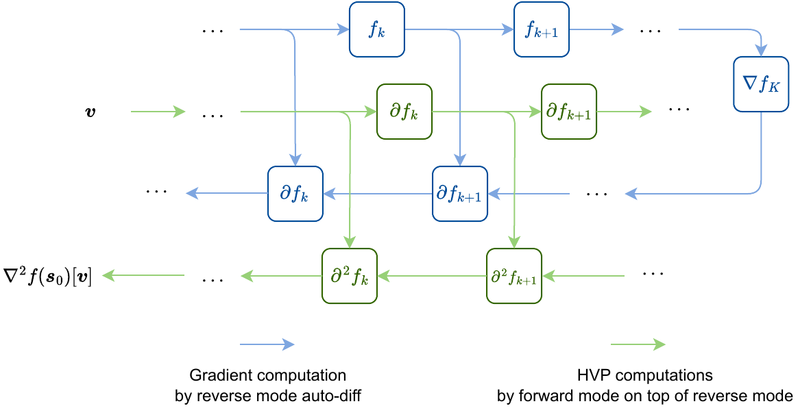
Figure 9.3: Computation graph for computing the HVP $\nabla^2 f(\w)[\v]$ by using forward mode on top of reverse mode. The forward mode naturally follows the computations done for the gradient, except that it passes through the derivatives of the intermediate operations.

With this in mind, following a similar calculation as for Table 8.1, we obtain the following results. We assume that each $\partial f_k(\s_{k-1})$ is a dense linear operator, so that its application has the same cost as a matrix-vector multiplication. For the memory complexity, we consider that the inputs of each operation are saved to compute the required derivatives in the backward passes.

Reverse on reverse: $O(KP^2)$ time and $O(KP)$ space.
Forward on reverse: $O(KP^2)$ time and $O(KP)$ space.
Reverse on forward: $O(KP^2)$ time and $O(KP)$ space.
Forward on forward: $O(KP^3)$ time and $O(3P)$ space for the $P$ JVPs with $\e_1,\dots,\e_P$ .

We see that, for chains of functions, “reverse on reverse”, “forward on reverse” and “reverse on forward” all have similar time complexities up to some constant factors. Using reverse mode on top of reverse mode requires storing the information backpropagated, i.e., the $\r_k$ (resp. the information forwarded, i.e., the $\t_k$ in Fig. 8.1), to perform the final reverse pass. By using forward mode on top of reverse mode, this additional cost is not incurred, making it slightly less memory expensive. In addition, reverse mode on top of reverse mode induces a few additional summations due to the branching and merge operations depicted in Fig. 9.2. The same holds when using reverse on top of forward as we cannot avoid fan-in operations (this time of the form $\s_{k-1}, \t_{k-1} \mapsto \partial f_k(\s_{k-1})[\t_{k-1}]$ ). Unfortunately, “forward on forward” is prohibitively expensive.

To summarize, among the four approaches presented to compute HVPs, the forward-on-reverse mode is a priori the most preferable in terms of computational and memory complexities. Note, however, that computations of higher derivatives can benefit from dedicated autodiff implementations such as Taylor mode autodiff, that do not merely compose forward and reverse modes. For general functions $f$ , it is reasonable to benchmark the first three methods to determine which method is the best for the function at hand.

9.2 Gauss-Newton matrix

9.2.1 An approximation of the Hessian

The Hessian matrix $\nabla^2 L(\w)$ of a function $L \colon \cW \to \RR$ is often used to construct a quadratic approximation of $L(\w)$ , $L(\w + \v) \approx L(\w) + \langle \nabla L(\w), \v \rangle + \frac{1}{2} \langle \v, \nabla^2 L(\w)[\v] \rangle.$ Unfortunately, when $L$ is nonconvex, $\nabla^2 L(\w)$ is typically an indefinite matrix, which means that the above approximation is a nonconvex quadratic w.r.t. $\v$ . For instance, if $L = \ell \circ f$ with $\ell$ convex, then $L$ is convex if $f$ is linear, but it is typically nonconvex if $f$ is nonlinear. The (generalized) Gauss-Newton matrix is a principled alternative to the Hessian, which is defined for $L \coloneqq \ell \circ f$ .

Definition 9.1 (Gauss-Newton matrix)

Given a differentiable function $f: \cW \rightarrow \cM$ and a twice differentiable function $\ell:\cM \rightarrow \RR$ , the (generalized) Gauss-Newton matrix of the composition $L = \ell \circ f$ evaluated at a point $\w \in \cW$ is defined as $\gn (\ell \circ f)(\w) \coloneqq \partial f(\w)^* \nabla^2\ell(f(\w)) \partial f(\w).$

As studied in Section 17.2, the Gauss-Newton matrix is a key ingredient of the Gauss-Newton method. An advantage of the Gauss-Newton matrix is its positive semi-definiteness provided that $\ell$ is convex.

Proposition 9.1 (Positive semi-definiteness of the GN matrix)

If $\ell$ is convex, then $\gn(\ell \circ f)(\w)$ is positive semi-definite for all $f$ .

This means that the approximation $L(\w + \v) \approx L(\w) + \langle \nabla L(\w), \v \rangle + \frac{1}{2} \langle \v, \gn L(\w)[\v] \rangle$ is a convex quadratic w.r.t. $\v$ .

Using the chain rule, we find that the Hessian of $L = \ell \circ f$ decomposes into the sum of two terms (see also Proposition 9.7).

Proposition 9.2 (Approximation of the Hessian)

For $f$ and $\ell$ twice differentiable, we have $\begin{align*} \nabla^2 (\ell \circ f)(\w) & = \partial f(\w)^* \nabla^2 \ell(f(\w)) \partial f(\w) + \partial^2 f(\w)^* [\nabla \ell(f(\w))] \\ & = \gn(\ell \circ f)(\w) + \sum_{j=1}^{M} \nabla_j \ell(f(\w)) \nabla^2 f_j(\w). \end{align*}$ If $f$ is linear, then the Hessian and Gauss-Newton matrices coincide, $\nabla^2 (\ell \circ f)(\w) = \gn(\ell \circ f)(\w).$

The Gauss-Newton operator $\gn(\ell \circ f)$ can therefore be seen as an approximation of the Hessian $\nabla^2 (\ell \circ f)$ , with equality if $f$ is linear.

9.2.2 Gauss-Newton chain rule

A chain rule for computing the Hessian of a composition of two functions is presented in Proposition 9.7, but the formula is relatively complicated, due to the cross-terms. In contrast, a Gauss-Newton chain rule is straightforward.

Proposition 9.3 (Gauss-Newton chain rule)

$\begin{align*} \gn(\ell \circ f \circ g)(\w) = \partial g(\w)^* \gn(\ell \circ f)(g(\w)) \partial g(\w). \end{align*}$

9.2.3 Gauss-Newton vector product

As for the Hessian, we rarely need to materialize the full Gauss-Newton matrix in memory. Indeed, we can define the Gauss-Newton vector product (GNVP), a linear map for a direction $\v \in \cW$ , as $\gn (\ell \circ f)(\w)[\v] \coloneqq \partial f(\w)^* [\nabla^2\ell(f(\w)) [\partial f(\w)[\v]]], \tag{9.1}$ where $\nabla^2\ell(f(\w))[\u]$ is the HVP of $\ell$ , a linear map from $\cM$ to $\cM$ . The GNVP can be computed using the JVP of $f$ , the HVP of $\ell$ and the VJP of $f$ . Instantiating the VJP requires $1$ forward pass through $f$ , from which we get both the value $f(\w)$ and the adjoint linear map $\u \mapsto \partial f(\w)^*[\u]$ . Evaluating the VJP requires $1$ backward pass through $f$ . Evaluating the JVP requires $1$ forward pass through $f$ . In total, evaluating $\v \mapsto \gn(\ell \circ f)(\w)[\v]$ therefore requires $2$ forward passes and $1$ backward pass through $f$ .

9.2.4 Gauss-Newton matrix factorization

In this section, we assume $\cW \subseteq \RR^P$ and $\cM \subseteq \RR^M$ . When $\ell$ is convex, we know that the Gauss-Newton matrix is positive semi-definite and therefore it can be factorized into $\gn(\ell\circ f)(\w) = VV^\top$ for some $V \in \RR^{P \times R}$ , where $R \le \min\{P,M\}$ is the rank of the matrix. Such a decomposition can actually be computed easily from a factorization of the Hessian of $\ell$ . For instance, suppose we know the eigendecomposition of the Hessian of $\ell$ , $\nabla^2 \ell(f(\w)) = \sum_{i=1}^M \lambda_i \u_i \u_i^\top$ , where the $\u_i$ are the eigenvectors and the $\lambda_i \geq 0$ are the eigenvalues (which we know are non-negative due to positive semidefiniteness). Then, the Gauss-Newton matrix can be decomposed as $\begin{align*} \gn(\ell \circ f)(\w) & = \sum_{i=1}^M \lambda_i \partial f(\w)^*[\u_i] \u_i^\top\partial f(\w) \\ & = \sum_{i=1}^M \left(\sqrt{\lambda_i} \partial f(\w)^*[\u_i]\right) \left(\sqrt{\lambda_i} \partial f(\w)^*[\u_i]\right)^\top \\ & = \sum_{i=1}^M \v_i\v_i^\top \quad \mbox{where} \ \v_i \coloneqq \sqrt{\lambda_i}\partial f(\w)^*[\u_i]. \end{align*}$ Stacking the vectors $\v_i$ into a matrix $V = (\v_1, \ldots, \v_M)$ , we recover the factorization $\gn(\ell\circ f)(\w) = VV^\top$ . To form this decomposition, we need to perform the eigendecomposition of $\nabla^2 \ell(f(\w)) \in \RR^{M \times M}$ , which takes $O(M^3)$ time. We also need $M$ calls to the VJP of $f$ at $\w$ . Compared to the direct implementation in Eq. (9.1), the factorization, once computed, allows us to compute the Gauss-Newton vector product (GNVP) as $\gn (\ell \circ f)(\w)[\v] = V V^\top \v$ . The factorization only requires $P \times M$ memory, while the direct implementation in Eq. (9.1) requires us to maintain the intermediate computations of $f$ . The computation-memory trade-offs therefore depend on the function considered.

9.2.5 Stochastic setting

Suppose the objective function is of the form $L(\w; \x, \y) \coloneqq \ell(f(\w; \x); \y).$ With some slight abuse of notation, we then have that the Gauss-Newton matrix associated with a pair $(\x,\y)$ is $\gn L(\w; \x, \y) \coloneqq \partial f(\w; \x)^* \nabla^2 \ell(\thetav; \y) \partial f(\w; \x),$ where $\thetav \coloneqq f(\w; \x)$ . Given a distribution $\rho$ over $(\x,\y)$ pairs, the Gauss-Newton matrix associated with the averaged loss $L(\w) \coloneqq \EE_{X,Y \sim \rho} \left[L(\w; X, Y)\right]$ is then $\gn L(\w) = \EE_{X,Y \sim \rho}\left[\gn L(\w; X, Y)\right].$

9.3 Fisher information matrix

9.3.1 Definition using the score function

The Fisher information is a way to measure the amount of information in a random variable $S$ .

Definition 9.2 (Fisher information matrix)

The Fisher information matrix, or Fisher for short, associated with the negative log-likelihood $L(\w; S) = -\log q_{\w}(S)$ of a probability distribution $q_\w$ with parameters $\w$ is the covariance of the gradients of $L$ at $\w$ for $S$ distributed according to $q_\w$ , $\begin{align*} \fisher L (\w) &\coloneqq \mathbb{E}_{S \sim q_{\w}}[\nabla L(\w; S) \otimes \nabla L(\w; S)] \\ &= \mathbb{E}_{S \sim q_{\w}}[\nabla_\w \log q_{\w}(S) \otimes \nabla_\w \log q_{\w}(S)]. \end{align*}$ The gradient $\nabla_\w \log q_{\w}(S)$ is known as the score function.

As studied in Section 17.3, the Fisher information matrix is a key ingredient of the natural gradient descent method.

9.3.2 Link with the Hessian

Provided that the probability distribution is twice differentiable w.r.t. $\w$ with integrable second derivatives, the Fisher information matrix can also be expressed as the Hessian of the negative log-likelihood (Amari, 1998; Martens, 2020).

Proposition 9.4 (Connection with the Hessian)

The Fisher information matrix of the negative log-likelihood $L(\w; S) = -\log q_{\w}(S)$ satisfies $\begin{align*} \fisher L (\w) &= \mathbb{E}_{S \sim q_{\w}}[\nabla^2 L(\w; S)] = \mathbb{E}_{S \sim q_{\w}}[-\nabla_{\w}^2\log q_{\w}(S)]. \end{align*}$

Remark 9.1 (Empirical Fisher)

We emphasize that in the above definitions, $S$ is sampled from the model distribution $q_\w$ , not from the data distribution $\rho$ . That is, we have $\begin{align*} \fisher L (\w) &=\mathbb{E}_{S \sim q_{\w}}[\nabla_\w \log q_{\w}(S)\nabla_\w \log q_{\w}(S)^\top] \\ &\neq \mathbb{E}_{S \sim \rho}[\nabla_\w \log q_{\w}(S)\nabla_\w \log q_{\w}(S)^\top] \end{align*}$ The latter is sometimes called ambiguously the “empirical” Fisher, though this name has generated confusion (Kunstner et al., 2019).

9.3.3 Equivalence with the Gauss-Newton matrix

So far, we discussed the Fisher information for a generic random variable $S \sim q_\w$ . We now discuss the supervised probabilistic learning setting where $S = (X, Y)$ and where, using the product rule of probability, we define the PDF $q_\w(X, Y) \coloneqq \rho_X(X) p_\thetav(Y)$ , with the shorthand $\thetav \coloneqq f(\w; X)$ .

Proposition 9.5 (Fisher matrix in supervised setting)

Suppose $(X, Y) \sim q_\w$ where the PDF of $q_\w$ is $q_\w(X, Y) \coloneqq \rho_X(X) p_\thetav(Y)$ . In that case, the Fisher information matrix of the negative log-likelihood $L(\w; \x, \y)= -\log q_{\w}(\x, \y)$ decomposes as: $\begin{align*} \fisher L (\w) & = \mathbb{E}_{(X, Y) \sim q_\w}[ \nabla_\w \log q_\w(X, Y) \otimes \nabla_\w \log q_\w(X, Y) ] \\ & = \mathbb{E}_{X \sim \rho_X} \left[ \mathbb{E}_{Y\sim p_{\thetav}}\left[ \nabla_\w \log p_{\thetav}(Y) \otimes \nabla_\w \log p_{\thetav}(Y)\right] \right] \\ & = \mathbb{E}_{X \sim \rho_X} \left[ \partial f(\w; X)^* \fisher \ell(\thetav) \partial f(\w; X) \right], \end{align*}$ where we defined the shorthand $\thetav \coloneqq f(\w; X)$ and where we defined the negative log-likelihood loss $\ell(\thetav; Y) \coloneqq -\log p_\thetav(Y)$ .

When $p_\thetav$ is an exponential family distribution, we can show that the Fisher information matrix and the Gauss-Newton matrix are equivalent.

Proposition 9.6 (Equivalence between Fisher and Gauss-Newton)

If $p_\thetav$ is an exponential family distribution, then $\begin{align*} \fisher L(\w) &= \EE_{X \sim \rho_X} \EE_{Y \sim p_\thetav} [\nabla L(\w; X, Y) \otimes \nabla L(\w; X, Y)] \\ &= \EE_{X \sim \rho_X} \EE_{Y \sim p_\thetav} [\partial f(\w; X)^* (\nabla \ell(\thetav; Y) \otimes \nabla \ell(\thetav; Y)) \partial f(\w; X)] \\ &= \EE_{X \sim \rho_X} \EE_{Y \sim p_\thetav} [\partial f(\w; X)^* \nabla^2 \ell(\thetav; Y) \partial f(\w; X)] \\ &= \EE_{X,Y \sim \rho}\left[\gn L(\w; X, Y)\right], \end{align*}$ where $\rho_X(\x) \coloneqq \int \rho(\x, \y)d\y$ .

Proof

From Proposition 3.3, if $p_\thetav$ is an exponential family distribution, $\nabla^2 \ell(\thetav; \y)$ is actually independent of $\y$ . Using Bartlett’s second identity Eq. (12.3), we then obtain $\begin{align*} \nabla^2 \ell(\thetav; \cdot) &= \EE_{Y \sim p_\thetav} [\nabla^2 \ell(\thetav; Y)] \\ &= \EE_{Y \sim p_\thetav} [-\nabla^2_\thetav \log p_\thetav(Y)] \\ &= \EE_{Y \sim p_\thetav} [\nabla_\thetav \log p_\thetav(Y) \otimes \nabla_\thetav \log p_\thetav(Y)] \\ &= \EE_{Y \sim p_\thetav} [\nabla \ell(\thetav; Y) \otimes \nabla \ell(\thetav; Y)], \end{align*}$ where we used $\cdot$ to indicate that the result holds for all $\y$ . Plugging the result back in the Fisher information matrix concludes the proof. ◻

9.4 Inverse-Hessian vector product

9.4.1 Definition as a linear map

We will see in Section 17.1 that Newton’s method uses iterations as $\begin{align*} \w^{t+1} & = \w^t - \nabla^2 L(\w^t)^{-1}\nabla L(\w^t). \end{align*}$ The inverse is well-defined if for example $L$ is strictly convex. Otherwise, some additional regularization can be added. Newton’s method therefore requires access to inverse-Hessian vector products (IHVPs), as defined below.

Definition 9.3 (Inverse-Hessian vector product)

For a twice differentiable function $L:\RR^P \rightarrow \RR$ , we define the inverse-Hessian Vector Product (IHVP) of $L$ at $\w \in \RR^P$ as the linear map $\u \mapsto \nabla^2 L(\w)^{-1} \u,$ provided that it exists. In other words, it is the linear map which to $\u$ associates $\v$ such that $\nabla^2 L(\w) \v = \u$ .

9.4.2 Implementation with matrix-free linear solvers

Numerous direct methods exist to compute the inverse of a matrix, such as the Cholesky decomposition, QR decomposition and Gaussian elimination. However, these algorithms require accessing elementary entries of the matrix, while an autodiff framework gives access to the Hessian through HVPs. Fortunately, there exist so-called matrix-free algorithms, that can solve a linear system of equations $H[\v] = \u$ by only accessing the linear map $\v \mapsto H[\v]$ for any $\v$ . Among such algorithms, we have the conjugate gradient (CG) method, that applies for $H$ positive-definite, i.e., such that $\langle \v, H[\v]\rangle >0$ for all $\v \neq 0$ , or the generalized minimal residual (GMRES) method, that applies for any invertible $H$ . A longer list of solvers can be found in public software such as SciPy (Virtanen et al., 2020). The IHVP of a strictly convex function (ensuring that the Hessian is positive definite) can therefore be computed by instantiating CG on the HVP, $\nabla^2 L(\w)^{-1} \u \approx \mathrm{CG}(\nabla^2 L(\w)[\cdot], \u).$ Positive-definiteness of the Hessian is indeed guaranteed for strictly convex functions for example, while for generic nonconvex functions, such a property may be verified around a minimizer but not in general. The conjugate gradient method is recalled in Algorithm 9.1 in its simplest form. In theory, the exact solution of the linear system is found after at most $T= P$ iterations of CG, though in practice numerical errors may prevent one from getting an exact solution.

Algorithm 9.1: Conjugate gradient method

Inputs: linear map $H[\cdot]: \RR^P \rightarrow \RR^P$ , target $\u \in \RR^P$ , initialization $\v_0$ (default $\zeros$ ), number of iterations $T$ (default $P$ ), target accuracy $\varepsilon$ (default machine precision)

$\r_0 = \u - H[\v_0]$

$\p_0 = \r_0$

for $t=0, \ldots, T-1$ do

$\alpha_t = \frac{\langle \r_t, \r_t \rangle}{\langle \p_t, H [\p_t]\rangle}$

$\v_{t+1} = \v_t + \alpha_t \p_t$

$\r_{t+1} = \r_t - \alpha_t H[\p_t]$

if $\langle \r_{t+1}, \r_{t+1} \rangle \leq \varepsilon$ then break

$\beta_t = \frac{\langle \r_{t+1}, \r_{t+1} \rangle}{\langle \r_t, \r_t \rangle}$

$\p_{t+1} = \r_{t+1} + \beta_t \p_t$

Output: $\v_T$ , such that $H[\v_T] \approx \u$

9.4.3 Complexity

For a given matrix $H \in \RR^{P \times P}$ , solving $H \v = \u$ can be done with decomposition methods (LU, QR, Cholesky) in $O(P^3)$ time. For matrix-free methods such as CG or GMRES, the cost per iteration is $O(P^2)$ . Since they theoretically solve the linear system in $O(P)$ iterations, the cost to obtain an exact solution is theoretically the same, $O(P^3)$ .

However, CG or GMRES differ from decomposition methods in that they are iterative methods, meaning that, at each iteration, they get closer to a solution. Unlike decomposition methods, this means that we can stop them before an exact solution is found. In practice, the number of iterations required to find a good approximate solution depends on the matrix. Well conditioned matrices require only few iterations. Badly conditioned matrices lead to some numerical instabilities for CG, so that more than $P$ iterations may be needed to get a good solution. In contrast, decomposition methods proceed in two steps: first they build a decomposition of $H$ at a cost of $O(P^3)$ , and second they solve a linear system at a cost of $O(P^2)$ , by leveraging the structure. LU and QR decompositions are known to be generally more stable and are therefore often preferred in practice, when we can access entries of $H$ at no cost.

If we do not have access to the Hessian $H$ , but only to its HVP, accessing entries of $H$ comes at a prohibitive cost. Indeed, entries of $H$ can still be recovered from HVPs, since $\e_i^\top H \e_j = H_{i,j}$ , but accessing each row or column of $H$ costs one HVP (matrix-vector product). To access the information necessary to use a decomposition method, we therefore need $P$ calls to HVPs before being able to actually compute the solution. For the same number of calls, CG or GMRES will already have found an approximate solution. In addition, a CG method does not require storing the matrix in memory.

9.5 Second-order backpropagation

9.5.1 Second-order Jacobian chain rule

The essential ingredient to develop forward-mode and reverse-mode autodiff hinged upon the chain rule for composed functions, $h = g \circ f$ . For second derivatives, a similar rule can be obtained. To do so, we slightly abuse notation and denote $\partial^2 h(\w)^*[\u] \coloneqq \nabla^2 \langle h, \u \rangle(\w) \in \RR^{P \times P},$ where $h: \RR^P \rightarrow \RR^Q$ , $\w \in \RR^P$ , $\u \in \RR^Q$ , and where we recall the shorthand notation $\langle \u, h\rangle(\w) \coloneqq \langle \u, h(\w)\rangle$ . Moreover, we view the above quantity as a linear map. Strictly speaking, the superscript ${}^*$ is not a linear adjoint anymore, since $\v_1, \v_2 \mapsto \partial^2 h(\w)[\v_1, \v_2]$ is no longer linear but bilinear. However, this superscript plays the same role as the VJP, since it takes an output vector and returns the input derivatives that correspond to infinitesimal variations along that output vector.

Proposition 9.7 (Hessian chain rule)

For two twice differentiable functions $f: \RR^P \rightarrow \RR^M$ and $g: \RR^M \rightarrow \RR^Q$ , the second directional derivative of the composition $g \circ f$ is a bilinear map from $\RR^P\times \RR^P$ to $\RR^Q$ along input directions $\v_1, \v_2 \in \RR^P$ of the form $\begin{align*} \partial^2 (g\circ f)(\w)[\v_1, \v_2] & = \partial g(f(\w))[\partial^2 f(\w)[\v_1, \v_2]] \\ & \quad + \partial^2 g(f(\w))[\partial f(\w)[\v_1], \partial f(\w)[\v_2]]. \end{align*}$ The Hessian of the composition $g\circ f$ along an output direction $\u \in \RR^Q$ is, seen as a linear map, $\begin{align*} \partial^2 (g\circ f)(\w)^*[\u] & = \partial^2 f(\w)^* [\partial g(f(\w))^*[\u]] \tag{9.2}\\ & \quad + \partial f(\w)^* \partial^2 g(f(\w))^*[\u] \partial f(\w). \end{align*}$ For the composition of $f \colon \RR^P \to \RR^M$ with a scalar-valued function $\ell \colon \RR^M \to \RR$ , we have in matrix form $\begin{align*} \nabla^2 (\ell \circ f)(\w) & = \sum_{j=1}^M (\nabla \ell(f(\w)))_j \nabla^2 f_j(\w)\\ & \quad + \jac f(\w)^\top \nabla^2 \ell(f(\w)) \jac f(\w). \end{align*}$

Note that, while the Hessian is usually defined for scalar-valued functions $h \colon \RR^P \to \RR$ , the above definition is for a generalized notion of Hessian that works for any function $h \colon \RR^P \to \RR^Q$ .

The Hessian backpropagation rule in Eq. (9.2) reveals two terms. The first one $\partial^2 f(\w)^* [\partial g(f(\w))^*[\u]]$ simply computes the Hessian of the intermediate function along the output direction normally backpropagated by a VJP. The second term $\partial f(\w)^* \partial^2 g(f(\w))^*[\u] \partial f(\w)$ shows how intermediate first-order variations influence second-order derivatives of the output.

Example 9.1 (Composition with an elementwise nonlinear function)

Consider the element-wise application of a twice differentiable scalar-valued function $f(\x) = (f(x_i))_{i=1}^M$ followed by some twice differentiable function $\ell$ . Note that $\nabla^2 f_i(\x) = f''(x_i) \e_i\e_i^\top$ . Hence, the Hessian of the composition reads $\begin{align*} \nabla^2 (\ell\circ f)(\x) & = \sum_{i=1}^M (\nabla \ell(f(\x)))_i f''(x_i) \e_i\e_i^\top \\ & \quad + \Diag(f'(\x)) \nabla^2 \ell(f(\x)) \Diag(f'(\x)) \\ & = \Diag(\nabla \ell(f(\x)) \odot f''(\x))\\ & \quad + \nabla^2 \ell(f(\x)) \odot (f'(\x) f'(\x)^\top), \end{align*}$ where $f'(\x) \coloneqq (f'(x_i))_{i=1}^M$ and $f''(\x) \coloneqq (f''(x_i))_{i=1}^M$ .

Example 9.2 (Hessian of the composition with a linear function)

Consider a linear function $f(\W) = \W\x$ , for $\W\in \RR^{M\times D}$ , composed with some twice differentiable function $\ell: \RR^M \rightarrow \RR$ . From Proposition 9.7, we get, in terms of linear maps, $\begin{align*} \nabla^2 (\ell\circ f)(\W) = \partial f(\W)^* \nabla^2 \ell(f(\W)) \partial f(\W). \end{align*}$ As already noted in Section 2.3, we have that $\partial f(\W)[\V] = \V \x$ and $\partial f(\W)^*[\u] = \u \x^\top$ . Hence, the Hessian seen as a linear map reads $\begin{align*} \nabla^2 (\ell\circ f)(\W)[\V] & = \partial f(\W)^*[ \nabla^2 \ell(f(\W)) [\partial f(\W)[\V]]] & = \H \V \x\x^\top, \end{align*}$ where $\H \coloneqq \nabla^2 \ell(f(\W))$ .

9.5.2 Computation chains

For a simple computation chain $f = f_K\circ \ldots \circ f_1$ as in Section 8.1, the formula derived in Proposition 9.7 suffices to develop an algorithm that backpropagates the Hessian, as shown in Algorithm 9.2. Compared to Algorithm 8.2, we simply backpropagate both the vectors $\r_k$ and the matrices $\bm{R}_k$ using intermediate first and second derivatives.

Algorithm 9.2: Hessian backprop for computation chains

Functions: $\ell \circ f$ with $f \coloneqq f_K \circ \ldots \circ f_1$ ,

Inputs: input $\x$

Initialize and store $\s_0 \coloneqq \x$ ▷ Forward pass

for $k\coloneqq 1, \ldots, K$ do

Compute and store $\s_k \coloneqq f_k(\s_{k-1})$

Initialize $\r_K \coloneqq \nabla \ell(\s_K), \ \bm{R}_K \coloneqq \nabla^2 \ell(\s_K)$ ▷ Backward pass

for $k\coloneqq K, \ldots, 1$ do

Compute $\r_{k-1} \coloneqq \partial f_k(\s_{k-1})^*[\r_k]$

Compute $\bm{R}_{k-1} \coloneqq \partial^2 f_k(\s_{k-1})^*[\r_k] + \partial f_k(\s_{k-1})^* \bm{R}_k \partial f_k(\s_{k-1})$

Release $\s_{k-1}$ from memory

Outputs: $\ell(f(\x)) = \ell(\s_K)$ , $\nabla(\ell \circ f)(\x) = \r_0$ , $\nabla^2(\ell \circ f)(\x) = \bm{R}_0$

9.5.3 Fan-in and fan-out

For generic computation graphs (see Section 8.3), we saw that multi-input functions (fan-in) were crucial. For Hessian backpropagation in computation graphs, we therefore need to develop a similar formula.

Proposition 9.8 (Hessian chain rule for fan-in)

Consider $n+1$ twice differentiable functions $f_1, \ldots, f_n$ and $g$ with $f_i: \RR^P \rightarrow \RR^{M_i}$ and $g: \RR^{M_1} \times \ldots \times \RR^{M_n} \rightarrow \RR^Q$ . The Hessian of $g \circ f$ for $f(\w)= (f_1(\w), \ldots, f_n(\w))$ along an output direction $\u \in \RR^Q$ is given by $\begin{align*} \partial^2 (g \circ f)(\w)^*[\u] & = \sum_{i=1}^n \partial^2 f_i(\w)^*[ \partial_i g(f(\w))^*[\u]] \\ & \quad + \sum_{i, j=1}^n \partial f_i(\w)^* \partial^2_{i, j} g(f(\w))^*[\u] \partial f_j(\w). \end{align*}$

The gradient backpropagation expression for fan-in is simple because the functions $f_i$ are not linked by any path. In contrast, the Hessian backpropagation involves cross-product terms
$\partial f_i(\w)^* \partial^2_{i, j} g(f(\w))^*[\u] \partial f_j(\w)$ for $i \neq j$ . The nodes associated with the $f_i$ computations cannot be treated independently anymore.

On the other hand, developing a backpropagation rule for fan-out does not pose any issue, since each output function can be treated independently.

Proposition 9.9 (Hessian chain rule for fan-out)

Consider $n+1$ twice differentiable functions $g_1, \ldots, g_n$ and $f$ with $g_i: \RR^M \rightarrow \RR^{Q_i}$ and $f: \RR^{P} \rightarrow \RR^M$ . The Hessian of $g \circ f$ for $g(\y)= (g_1(\y), \ldots, g_n(\y))$ along a direction $\u = (\u_1, \ldots, \u_n) \in \RR^{Q_1} \times \ldots \times \RR^{Q_n}$ is given by $\begin{align*} \partial^2 (g \circ f)(\w)^*[\u] & = \sum_{i=1}^n \partial^2 f(\w)^*[ \partial g_i(f(\w))^*[\u_i]] \\ & \quad + \sum_{i=1}^n \partial f(\w)^* \partial^2 g_i(f(\w))^*[\u_i] \partial f(\w). \end{align*}$

9.6 Block diagonal approximations

Rather than computing the whole Hessian or Gauss-Newton matrices, we can consider computing block-diagonal or diagonal approximations, which are easier to invert. The approximation rules we present in this section build upon the Hessian chain rule studied in Section 9.5.

9.6.1 Feedforward networks

Recall the definition of a feedforward network: $\begin{align*} \s_0 &\coloneqq \x \\ \s_k &\coloneqq f_k(\s_{k-1}, \w_k) ~ \forall k \in \{1, \ldots, K\} \\ f(\x, \w) &\coloneqq \s_K, \end{align*}$ where $\w \coloneqq (\w_1, \dots, \w_K)$ . Rather than computing the entire Hessian of $\ell \circ f$ w.r.t. $\w$ , we can compute the Hessians w.r.t. each set of parameters $\w_k$ . For the case of computation chains, the Hessian backpropagation recursion we used in Algorithm 9.2 was $\bm{R}_{k-1} \coloneqq \partial^2 f_k(\s_{k-1})^*[\r_k] + \partial f_k(\s_{k-1})^* \bm{R}_k \partial f_k(\s_{k-1}).$ Extending this recursion to the feedforward network case, we obtain, starting from $\r_K \coloneqq \nabla \ell(\s_K)$ and $\bm{R}_K \coloneqq \nabla^2 \ell(\s_K)$ , $\begin{align*} \r_{k-1} &\coloneqq \partial f_k(\s_{k-1}, \w_k)^*[\r_k] \\ \begin{pmatrix} \bm{R}_{k-1} & \sim \\ \sim & \bm{H}_k \end{pmatrix} & \coloneqq \partial^2 f_k(\s_{k-1}, \w_k)^*[\r_k] \\ & \quad + \partial f_k(\s_{k-1}, \w_k)^* \bm{R}_k \partial f_k(\s_{k-1}, \w_k), \end{align*}$ where we used $\sim$ to indicate that these blocks are not used. The Hessians w.r.t. each set of parameters are then $\begin{align*} \bm{R}_0 &= \nabla_{\x\x}^2 (\ell\circ f)(\x, \w) \\ \H_1 &= \nabla_{\w_1\w_1}^2(\ell\circ f)(\x, \w) \\ &\vdots \\ \H_K &= \nabla_{\w_K\w_K}^2(\ell\circ f)(\x, \w). \end{align*}$ The validity of this result stems from the fact that we can view the Hessian w.r.t. $\w_k$ as computing the Hessian w.r.t. $\w_k$ of $\tilde{f}_K \circ \ldots \circ \tilde{f}_{k+1} \circ f_k(\s_{k-1}, \w_k)$ where $\tilde{f}_i \coloneqq f_i(\cdot, \w_i)$ , for $i \in \{k+1,\dots,K\}$ . As the computations of the block-wise Hessians share most of the computations, they can be evaluated in a single backward pass just as the gradients.

Example 9.3 (Block-wise computation of the Gauss-Newton matrix)

Our blockwise backpropagation scheme can readily be adapted for the Gauss-Newton matrix as $\begin{align*} \begin{pmatrix} \bm{R}_{k-1} & \sim \\ \sim & \G_k \end{pmatrix} & \coloneqq \partial f_k(\s_{k-1}, \w_k)^* \bm{R}_k \partial f_k(\s_{k-1}, \w_k), \end{align*}$ starting from $\bm{R}_K \coloneqq \nabla^2 \ell(\s_K)$ . The outputs $\bm{R}_0, \G_1, \ldots, \G_K$ give a block-wise approximation of the Gauss-Newton matrix.

Now, consider a simple multilayer perceptron such that $f_k(\s_{k-1}, \w_k) \coloneqq \a(\W_k \s_{k-1}) \quad \text{with} \quad \w_k \coloneqq \Vec(\W_k)$ Using Example 9.2 and Example 9.1 adapted to the Gauss-Newton matrix, we can compute the block-wise decomposition of the Gauss-Newton matrix as, for $k=K, \ldots, 1$ , $\begin{align*} \bm{R}_{k-1} &\coloneqq \W_k^\top \J_k \W_k \\ \J_k &\coloneqq \bm{R}_k \odot (\a'(\W_k \s_{k-1})\a'(\W_k\s_{k-1})^\top ) \\ \G_k &\coloneqq \J_k \otimes \s_{k-1} \s_{k-1}^\top \end{align*}$ starting from $\bm{R}_K \coloneqq \nabla^2 \ell(\s_K)$ . The outputs $\G_1, \ldots, \G_K$ correspond to the block-wise elements of the Gauss-Newton matrix of $f$ for the vectorized weights $\w_1, \ldots, \w_K$ . Similar computations were done in KFRA (Botev et al., 2017) and BackPack (Dangel et al., 2019).

9.6.2 Computation graphs

For generic computation graphs, consider a function $f(\x, \w)$ defined by, denoting $i_1, \ldots, i_{p_k} \coloneqq \parent(k)$ , $\s_k \coloneqq f_k(\s_{i_1}, \ldots, \s_{i_{p_k}}) \quad \forall k \in \{1, \ldots, K\}$ such that $f(\x, \w) = \s_K$ , and $k$ is following a topological ordering of the graph (see Section 8.3). We can consider the following backpropagation scheme, for $k = K, \ldots, 1$ and $j \in \parent(k)$ $\begin{align*} \r_{i_j} & \leftarrow \r_{i_j} + \partial_j f_k(\s_{i_1}, \ldots, \s_{i_{p_k}})^*[\r_k] \tag{9.3}\\ \bm{R}_{i_j} & \leftarrow \bm{R}_{i_j} + \partial^2_{jj} f_k(\s_{i_1}, \ldots, \s_{i_{p_k}})^*[\r_k] \\ & \quad + \partial_j f_k(\s_{i_1}, \ldots, \s_{i_{p_k}})^* \bm{R}_k \partial_j f_k(\s_{i_1}, \ldots, \s_{i_{p_k}}), \tag{9.4}\end{align*}$ starting from $\bm{R}_K \coloneqq \nabla^2 \ell(\s_K)$ and $\r_K \coloneqq \nabla \ell(\s_K)$ . Recall that for multiple inputs, the chain rule presented in Proposition 9.8 involves the cross-derivatives. For this reason the backpropagation scheme in Eq. (9.3) only computes an approximation. For example, one can verify that using Eq. (9.3) to compute the Hessian of $\ell(f_1(\w), f_2(\w))$ does not provide an exact expression for the Hessian of $f$ . This scheme is easy to implement and may provide a relevant proxy for the Hessian.

9.7 Diagonal approximations

Similarly to the idea of designing a backpropagation scheme that approximates blocks of the Hessian, we can design a backpropagation scheme that approximates the diagonal of the Hessian. The approach was originally proposed by Becker and Le Cun (1988) for feedforward networks, but our exposition, new to our knowledge, has the benefit that it naturally extends to computational graphs, as we shall see.

9.7.1 Computation chains

The idea stems from modifying the Hessian backpropagation rule in Proposition 9.7 to only keep the diagonal of the Hessian. Formally, given a matrix $\M \in \RR^{D \times D}$ , we denote by $\diag(\M) = (\M_{ii})_{i=1}^D \in \RR^{D}$ the vector of diagonal entries of $\M$ , and for a vector $\m\in \RR^D$ , we denote $\Diag(\m) = \sum_{i=1}^D m_i\e_i\e_i^\top$ the diagonal matrix with entries $m_i$ . For the backpropagation of the Hessian of $\ell \circ f_K \circ \ldots \circ f_1$ , we see from Algorithm 9.2 that $\diag(\H_{k-1})$ can be expressed in terms of $\H_k$ as $\begin{align*} \diag(\H_{k-1}) = & \diag(\partial^2 f_k(\s_{k-1})^* \r_k) \\ & + \diag(\jac f_k(\s_{k-1})^* \H_k \jac f_k(\s_{k-1})). \end{align*}$ Unfortunately, that recursion needs access to the whole Hessian $\H_k$ , and would therefore be too expensive. A natural idea is to modify the recursion to approximate $\diag(\H_k)$ by backpropagating vectors: $\begin{align*} \d_{k-1} \coloneqq &\diag(\partial^2 f_k(\s_{k-1})^* \r_k) \\ & + \diag(\jac f_k(\s_{k-1})^* \Diag(\d_k) \jac f_k(\s_{k-1})). \end{align*}$ The diagonal matrix $\Diag(\d_k)$ serves as a surrogate for $\H_k$ . Each iteration of this recursion can be computed in linear time in the output dimension $D_k$ since $\begin{align*} d_{k-1,i} = &\sum_{j=1}^{D_k} r_{k,j} \cdot \partial_{i,i}^2 f_{k,j}(\s_{k-1}) + \sum_{j=1}^{D_k} d_{k,j} (\partial_i f_{k,j}(\s_{k-1}))^2. \end{align*}$ To initialize the recursion, we can set $\d_K \coloneqq \diag(\nabla^2 \ell(\s_K))$ . As an alternative, as proposed by Elsayed and Mahmood (2022), if $\H_K$ has a simple form, we can use $\nabla^2\ell(\s_K)$ instead of $\Diag(\d_K)$ at the first iteration. This is the case for instance if $f_K$ is a cross-entropy loss. The recursion is repeated until we obtain the approximate diagonal Hessian $\d_0 \approx \diag(\nabla^2 (\ell\circ f)(\x))$ . The gradients $\r_k$ , needed to compute $\d_k$ , are computed along the way and the algorithm can therefore also return $\r_0 = \nabla (\ell\circ f)(\x)$ .

9.7.2 Computation graphs

Although this diagonal approximation was originally derived for feedforward networks by Becker and Le Cun (1988), it is straightforward to generalize it to computation graphs. Namely, for a function $f(\x, \w)$ decomposed along a computation graph, we can backpropagate a diagonal approximation in reverse topological order as $\begin{align*} \r_{i_j} & \leftarrow \r_{i_j} + \partial_j f_k(\s_{i_1}, \ldots, \s_{i_{p_k}})^*[\r_k] \\ \d_{i_j} & \leftarrow \d_{i_j} + \diag(\partial^2_{jj} f_k(\s_{i_1}, \ldots, \s_{i_{p_k}})^*[\r_k]) \\ & \quad + \diag( \partial_j f_k(\s_{i_1}, \ldots, \s_{i_{p_k}})^* \Diag(\d_k) \partial_j f_k(\s_{i_1}, \ldots, \s_{i_{p_k}}) ), \tag{9.5}\end{align*}$ for $j \in \parent(k)$ , starting from $\r_K = \nabla \ell(\s_K)$ and $\d_K = \diag(\nabla^2 \ell(\s_K))$ or $\Diag(\d_K) = \nabla^2 \ell(\s_K)$ . To implement such an algorithm, each elementary function in the computational graph needs to be augmented with an oracle that computes the Hessian diagonal approximation of the current function, given the previous ones. An example with MLPs is presented in Example 9.4.

Example 9.4 (Hessian diagonal approximation for MLPs)

Consider a multilayer perceptron $\begin{align*} \s_{k} &\coloneqq \a_k(\W_k \s_{k-1}) \quad \forall k \in \{1,\dots,K\}\\ f(\w, \x) &\coloneqq \s_K \end{align*}$ starting from $\s_0 = \x$ . Here $\a_k$ is the element-wise activation function (potentially the identity) and $\w$ encapsulates the weight matrices $\W_1, \ldots, \W_K$ . We consider the derivatives w.r.t. the flattened matrices, so that gradients and diagonal approximations w.r.t. these flattened quantities are vectors. The backpropagation scheme (9.5) then reduces to, denoting $\t_k = \W_k \s_{k-1}$ , $\begin{align*} \r_{k-1} &\coloneqq \W_k^\top (\a'(\t_k) \odot \r_k) \\ \g_k &\coloneqq \Vec((\a'(\t_k) \odot \r_k) \s_{k-1}^\top) \\ \deltav_k &\coloneqq \r_k \odot \a''(\t_k) + \d_k\odot \a'(\t_k)^2 \\ \d_{k-1} &\coloneqq \left(\sum_{j=1}^{D_k} \W_{k, j i}^2 \delta_{k, j}\right)_{i=1}^{D_{k-1}} \\ \h_k &\coloneqq \Vec(\deltav_k (\s_{k-1}^2)^\top) \end{align*}$ starting from $\r_K = \nabla \ell(\s_K)$ and, e.g., $\d_K = \diag(\nabla^2 \ell(\s_K))$ . The algorithm returns $\g_1, \ldots, \g_K$ as the gradients of $f$ w.r.t. $\w_1, \ldots, \w_K$ , with $\w_i = \Vec(\W_i)$ , and $\h_1, \ldots, \h_K$ as the diagonal approximations of the Hessian w.r.t. $\w_1, \ldots, \w_K$ .

9.8 Randomized estimators

In this section, we describe randomized estimators of the diagonal of the Hessian or Gauss-Newton matrices.

9.8.1 Girard-Hutchinson estimator

We begin with a generic estimator, originally proposed for trace estimation by Girard (1989) and extended by Hutchinson (1989). Let $\A \in \RR^{P \times P}$ be an arbitrary square matrix, whose matrix-vector product (matvec) is available. Suppose $\omegav \in \RR^P$ is an isotropic random vector, i.e., such that $\EE_{\omegav \sim p}[\omegav \omegav^\top] = I$ . For example, two common choices are the Rademacher distribution $p = \mathrm{Uniform}(\{-1, 1\}^P)$ and the standard normal distribution $p = \mathrm{Normal}(\zeros, I_P)$ . Then, we have $\EE_{\omegav \sim p}[\langle \omegav, \A \omegav \rangle] = \Tr(\A).$ Applications include generalized cross-validation, computing the Kullback-Leibler divergence between two Gaussians, and computing the derivatives of the log-determinant.

The approach can be extended (Baston and Nakatsukasa, 2022; Bekas et al., 2007; Hallman et al., 2023) to obtain an estimator of the diagonal of $\A$ , $\EE_{\omegav \sim p}[\omegav \odot \A \omegav] = \diag(\A),$ where $\odot$ denotes the Hadamard product (element-wise multiplication). This suggests that we can use the Monte-Carlo method to estimate the diagonal of $\A$ , $\diag(\A) \approx \frac{1}{S} \sum_{i=1}^S \omegav_i \odot \A \omegav_i,$ with equality as $S \to \infty$ , since the estimator is unbiased. Since, as reviewed in Section 9.1 and Section 9.2, we know how to multiply efficiently with the Hessian and the Gauss-Newton matrices, we can apply the technique with these matrices. The variance is determined by the number $S$ of samples drawn and therefore by the number of matvecs performed. More elaborate approaches have been proposed to further reduce the variance (Epperly et al., 2023; Meyer et al., 2021).

9.8.2 Bartlett estimator for the factorization

Suppose the objective function is of the form $L(\w; \x, \y) \coloneqq \ell(f(\w; \x); \y)$ where $\ell$ is the negative log-likelihood $\ell(\thetav; \y) \coloneqq -\log p_\thetav(\y)$ of an exponential family distribution, and $\thetav \coloneqq f(\w; \x)$ , for some network $f$ . We saw from the equivalence between the Fisher and Gauss-Newton matrices in Proposition 9.6 (which follows from the Bartlett identity) that $\begin{align*} \gn L(\w; \x, \cdot) &= \EE_{Y \sim p_\thetav} [\partial f(\w; \x)^* \nabla \ell(\thetav; Y) \otimes \nabla \ell(\thetav; Y) \partial f(\w; \x)] \\ &= \EE_{Y \sim p_\thetav} [\nabla L(\w; \x, Y) \otimes \nabla L(\w; \x, Y)], \end{align*}$ where $\cdot$ indicates that the result holds for any value of the second argument. This suggests a Monte-Carlo scheme $\begin{align*} \gn L(\w; \x, \cdot) \approx \frac{1}{S} \sum_{j=1}^S [\nabla L(\w; \x, \y_{i_j}) \otimes \nabla L(\w; \x, \y_{i_j})] \end{align*}$ where $\y_{i_1},\dots,\y_{i_S} \sim p_\thetav$ and $\thetav = f(\w, \x)$ . In words, we can approximate the Gauss-Newton matrix with $S$ gradient computations. This factorization can also be used to approximate the GNVP in Eq. (9.1).

9.8.3 Bartlett estimator for the diagonal

Following a similar approach, we obtain $\diag(\gn L(\w; \x, \cdot)) = \EE_{Y \sim p_\thetav} [\nabla L(\w; \x, Y) \odot \nabla L(\w; \x, Y)],$ where $\odot$ indicates the element-wise (Hadamard) product. Using a Monte-Carlo scheme, sampling $\y_{i_1}, \dots, \y_{i_S}$ from $p_\thetav$ , we therefore obtain $\diag(\gn L(\w; \x, \cdot)) \approx \frac{1}{S} \sum_{j=1}^S \nabla L(\w; \x, \y_{i_j}) \odot \nabla L(\w; \x, \y_{i_j}),$ with equality when all labels in the support of $p_\thetav$ have been sampled. That estimator, used for instance in (Wei et al., 2020, Appendix C.1.), requires access to individual gradients evaluated at the sampled labels. Another possible estimator of the diagonal is given by $\begin{align*} &\frac{1}{S} \diag(\gn L(\w; \x, \cdot)) \\ =& \EE_{Y_1, \dots, Y_S \sim p_\thetav} \left[\nabla \frac{1}{S} \sum_{i=1}^S L(\w; \x, Y_i) \odot \nabla \frac{1}{S} \sum_{i=1}^S L(\w; \x, Y_i)\right]. \end{align*}$ Letting $\gamma_i \coloneqq \nabla L(\w; \x, Y_i)$ , this follows from $\begin{align*} \EE\left[\left(\sum_i \gamma_i\right) \odot \left(\sum_j \gamma_j\right)\right] &= \EE\left[\sum_i \gamma_i \odot \gamma_i + \sum_{i \neq j} \gamma_i \odot \gamma_j\right] \\ &= \EE\left[\sum_i \gamma_i \odot \gamma_i\right] \end{align*}$ where we used that $\EE[\gamma_i \odot \gamma_j] = \EE[\gamma_i] \odot \EE[\gamma_j] = \zeros$ since $\gamma_i$ and $\gamma_j$ are independent variables for $i \neq j$ and have zero mean, from Bartlett’s first identity Eq. (12.2). We can then use the Monte-Carlo method to obtain $\begin{align*} \frac{1}{S} \diag(\gn L(\w; \x, \cdot)) \approx \left(\nabla \frac{1}{S} \sum_{j=1}^S L(\w; \x, \y_{i_j})\right) \odot \left(\nabla \frac{1}{S} \sum_{j=1}^S L(\w; \x, \y_{i_j})\right), \end{align*}$ with equality when all labels in the support of $p_\thetav$ have been sampled. This estimator can be more convenient to implement, since it only needs access to the gradient of the averaged losses. However, it may suffer from higher variance. A special case of this estimator is used by Liu et al. (2023), where they draw only one $\y$ for each $\x$ .

9.9 Summary

By using a Hessian chain rule, we can develop a “Hessian backpropagation”. While it is reasonably simple for computation chains, it becomes computationally prohibitive for computation graphs, due to the cross-product terms occurring with fan-in.
A better approach is to use Hessian-vector products (HVPs). We saw that there are four possible methods to compute HVPs, but the forward-on-reverse method is a priori the most efficient. Similarly to computing gradients, computing HVPs is only a constant times more expensive than evaluating the function itself.
The Gauss-Newton matrix associated with the composition $\ell \circ f$ can be seen as an approximation of the Hessian. It is a positive semidefinite matrix if $\ell$ is convex, and can be used to build a principled quadratic approximation of a function. It is equivalent to the Fisher information matrix in the case of exponential families. Gauss-Newton-vector products can be computed efficiently, like HVPs.
We also described other approximations, such as (block) diagonal approximations, and randomized estimators.