Control flows, such as conditionals or loops, are an essential part of computer programming, as they allow us to express complex programs. It is therefore natural to ask whether these constructs can be included in a differentiable program. This is what we study in this chapter.
5.1 Comparison operators
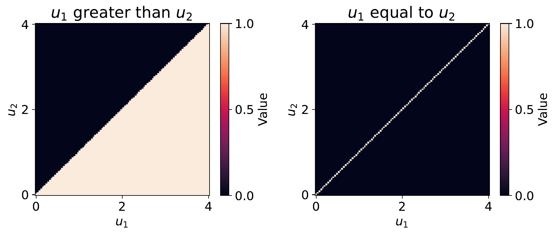
Control flows rely on comparison operators, a.k.a. relational operators. Formally, we can define a comparison operator π=op(u1,u2) as a function from u1∈R and u2∈R to π∈{0,1}. The binary (Boolean) output π can then be used within a conditional statement (see Section 5.6, Section 5.7) to decide whether to execute one branch or another. We define the following operators, illustrated in Fig. 5.1:
greater than:gt(u1,u2):={10 if u1≥u2 otherwise =step(u1−u2)
less than:lt(u1,u2):={10 if u1≤u2 otherwise =step(u2−u1)
equal:eq(u1,u2):={10 if ∣u1−u2∣=0 otherwise =gt(u2,u1)⋅gt(u1,u2)=step(u2−u1)⋅step(u1−u2)
not equal:neq(u1,u2):={10 if ∣u1−u2∣>0 otherwise =1−eq(u1,u2)=1−step(u2−u1)⋅step(u1−u2),
where step:R→{0,1} is the Heaviside step functionstep(u):={10 if u≥0 otherwise. The Heaviside step function is piecewise constant. At u=0, the function is discontinuous. At u=0, it is continuous and has null derivative. Since the comparison operators we presented are all expressed in terms of the step function, they are all continuous and differentiable almost everywhere, with null derivative. Therefore, while their derivatives are well-defined almost everywhere, they are uninformative and prevent gradient backpropagation.
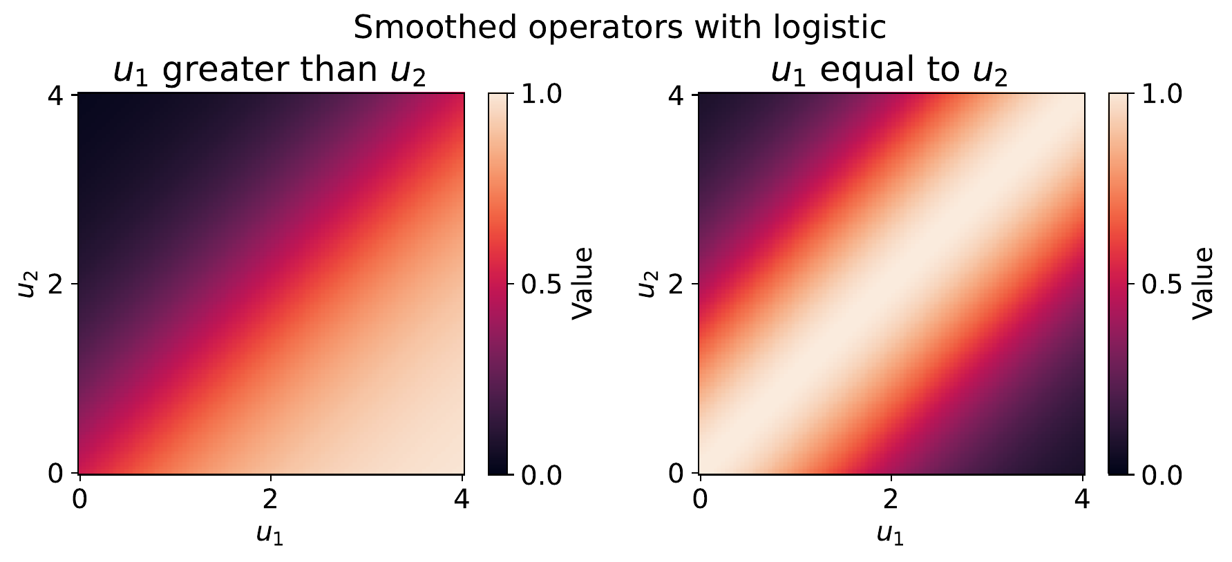
Figure 5.1: The greater than and equal to operators are discontinuous functions, leading to black or white pictures. They can be smoothed with appropriate approximations of the Heaviside step function.
5.2 Soft inequality operators
5.2.1 Heuristic definition
To obtain a continuous relaxation of inequality operators, we can heuristically replace the step function in the expression of “greater than” and “less than” by a sigmoid function sigmoidσ, where σ>0 is a scaling parameter. Such a sigmoid function should satisfy the following properties:
sigmoidσ(−u)=1−sigmoidσ(u),
limu→∞sigmoidσ(u)=1,
limu→−∞sigmoidσ(u)=0,
sigmoidσ(0)=21.
Two examples of sigmoids satisfying the aforementioned properties are the logistic function (the CDF of the standard logistic distribution) sigmoidσ(u):=logisticσ(u):=1+e−u/σ1∈(0,1) and the standard Gaussian’s CDF, defined in Eq. (3.1), sigmoidσ(u):=Φ(u/σ). We may then define the soft “greater than” gt(μ1,μ2)=step(μ1−μ2)≈sigmoidσ(μ1−μ2)=:gtσ(μ1,μ2) and the soft “less than” lt(μ1,μ2)=step(μ2−μ1)≈sigmoidσ(μ2−μ1)=:ltσ(μ1,μ2)=1−sigmoidσ(μ1−μ2)=1−gtσ(μ1,μ2). In the limit, we have that sigmoidσ(μ1−μ2)→1 when μ1−μ2→∞. In the limit, sigmoidσ therefore outputs a value of 1 if μ1 and μ2 are infinitely apart. Besides the logistic function and the standard Gaussian’s CDF, other sigmoid functions are possible, as discussed in Section 13.6. In particular, with sparse sigmoids, there exists a finite value τ such that μ1−μ2≥τ⟹sigmoidσ(μ1−μ2)=1.
5.2.2 Stochastic process perspective
When the sigmoid used to replace the step function is the logistic function or the standard Gaussian’s CDF, we can revisit the previous heuristic definition of gtσ(μ1,μ2) and ltσ(μ1,μ2) from a more formal perspective. Indeed, to real values μ1∈R and μ2∈R, we can associate random variables U1∼pμ1,σ1andU2∼pμ2,σ2, thereby forming a stochastic process (we assume that σ1 and σ2 are fixed). Alternatively, we can also write (U1,U2)∼pμ1,σ1⊗pμ2,σ2, where for two distributions p1 and p2, we denote by p1⊗p2 their outer product (p1⊗p2)(u1,u2):=p1(u1)p2(u2). We can then define gtσ(μ1,μ2)=E[gt(U1,U2)]=E[step(U1−U2)]=P(U1−U2≥0)=P(U2−U1≤0)=FU2−U1(0), where FX is the cumulative distribution function (CDF) of the random variable X, and σ is a function of σ1 and σ2. Similarly, we obtain ltσ(μ1,μ2)=E[lt(U1,U2)]=E[step(U2−U1)]=P(U1−U2≤0)=FU1−U2(0). We see that the soft inequality operators are based on the CDF of the difference between U1 and U2.
For location-scale family distributions (Section 12.4.1), from a perturbation perspective, we can also define noise variables Z1∼p0,1 and Z2∼p0,1 such that U1=μ1+σ1Z1 and U2=μ2+σ2Z2 (Section 12.4.1). We then have gtσ(μ1,μ2)ltσ(μ1,μ2)=E[gt(μ1+σ1Z1,μ2+σ2Z2)]=E[lt(μ1+σ1Z1,μ2+σ2Z2)].
Gaussian case
When U1∼Normal(μ1,σ12) and U2∼Normal(μ2,σ22), we have U1−U2∼Normal(μ1−μ2,σ12+σ22).(5.1) Denoting Φ the standard Gaussian’s CDF, we then obtain gtσ(μ1,μ2)ltσ(μ1,μ2)=FU2−U1(0)=Φ(σ0−(μ2−μ1))=Φ(σμ1−μ2)=FU1−U2(0)=Φ(σ0−(μ1−μ2))=Φ(σμ2−μ1), where σ:=σ12+σ22. The corresponding distribution for Z1 and Z2 is Gaussian noise.
Logistic case
When U1∼Gumbel(μ1,σ) and U2∼Gumbel(μ2,σ), we have U1−U2∼Logistic(μ1−μ2,σ).(5.2) We then obtain (see also Proposition 14.3) gtσ(μ1,μ2)ltσ(μ1,μ2)=logistic(σμ1−μ2)=logistic(σμ2−μ1). The corresponding distribution for Z1 and Z2 is Gumbel noise.
Recovering hard inequality operators
We easily recover the “hard” inequality operator by gt(μ1,μ2)=E[gt(U1,U2)], where Ui∼δμi and where δμi is the delta distribution that assigns a probability of 1 to μi.
5.3 Soft equality operators
5.3.1 Heuristic definition
The equality operator eq(μ1,μ2) can be seen as an extreme kind of similarity function between numbers, that can only output the values 0 or 1. To define soft equality operators, a natural idea is therefore to replace the equality operator by a more general similarity function. A similarity function should achieve its maximum at μ1=μ2 and it should decrease as μ1 and μ2 move apart. A common family of similarity functions are kernels. Briefly, a kernel k(μ1,μ2) can be seen as the inner product k(μ1,μ2):=⟨ϕ(μ1),ϕ(μ2)⟩ between the embeddings ϕ(μ1) and ϕ(μ2) of μ1 and μ2 in some (potentially infinite-dimensional) space H, a reproducing kernel Hilbert space to be precise; see Schölkopf and Smola (2002; Shawe-Taylor and Cristianini, 2004) for an in-depth review of kernels. To obtain a similarity measure between 0 and 1 approximating the equality operator, we can normalize to obtain eq(μ1,μ2)≈k(μ1,μ1)k(μ2,μ2)k(μ1,μ2)=∥ϕ(μ1)∥∥ϕ(μ2)∥⟨ϕ(μ1),ϕ(μ2)⟩, where ∥ϕ(μ)∥:=⟨ϕ(μ),ϕ(μ)⟩=κ(μ,μ). This is the cosine similarity between ϕ(μ1) and ϕ(μ2).
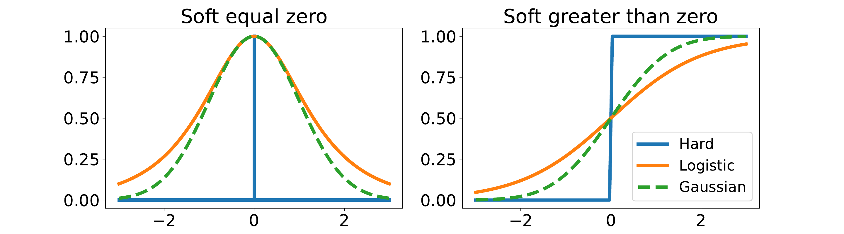
A particular kind of kernel is isotropic kernels of the form k(μ1,μ2):=κ(μ1−μ2), that depend only on the difference between inputs. When the kernel has a scale parameter σ>0, we use the notation κσ. We can then define a soft equality operator as eq(μ1,μ2)≈eqσ(μ1,μ2):=κσ(0)κσ(μ1−μ2). Several isotropic kernels can be chosen such as the Gaussian kernelκσ(t):=exp(−2σ2t2) or the logistic kernelκσ(t):=sech2(2σt), where we defined the hyperbolic secant sech(u):=2/(exp(u)+exp(−u)). As their names suggest, these kernels arise naturally from a probabilistic perspective, that we present below.
The soft equality operators obtained with these kernels are illustrated in Fig. 5.2. Intuitively, we replaced a bar located at μ1=μ2 with a bump function. The soft equality operator obtained with the logistic kernel coincides with the expression Petersen et al. (2021) arrive at (see their Eq. 9), in a different manner.
Figure 5.2: Soft equality and soft greater than operators can be defined as normalized kernels (PDF) and as CDF functions, respectively.
5.3.2 Stochastic process perspective
We again adopt the stochastic process perspective, in which we associate random variables U1∼pμ1,σandU2∼pμ2,σ to real values μ1∈R and μ2∈R. However, to handle the equality operator, we cannot simply use the expectation of eq(U1,U2) since E[eq(U1,U2)]=P(U1=U2)=0,U1 and U2 being independent continuous variables. While we cannot use the probability of U1=U2, or equivalently of U1−U2=0, we can consider using the probability density function (PDF) fU1−U2 of U1−U2 evaluated at 0. To ensure that the maximum is achieved at 0 with value 1, we can normalize the PDF to define eqσ(μ1,μ2)=fU0(0)fU1−U2(0), where U0∼p0,σ (we assume that fU0 attains its maximum at 0). It is well-known that the PDF of the sum of two random variables is the convolution of their respective PDFs. We therefore have fU1−U2(t)=(fU1∗f−U2)(t)=∫−∞∞fU1(τ)f−U2(t−τ)dτ. In particular, with t=0, if fX is the PDF of a location-scale family distributed random variable, we obtain fU1−U2(0)=(fU1∗f−U2)(0)=∫−∞∞fU1(τ)f−U2(−τ)dτ=∫−∞∞fU1(τ)fU2(τ)dτ:=⟨fU1,fU2⟩:=κ(μ1,μ2). We indeed recover an inner product and therefore a kernel.
CDF and PDF of absolute difference
While P(U1=U2)=0, we can also consider using P(∣U1−U2∣≤ε)=F∣U1−U2∣(ε) as an alternative notion of soft equality. For any random variable X, we have F∣X∣(x)=P(∣X∣≤x)=P(−x≤X≤x)=P(X≤x)−P(X≤−x)=FX(x)−FX(−x). Therefore, P(∣U1−U2∣≤ε)=FU1−U2(ε)−FU1−U2(−ε). We can also derive the PDF of ∣X∣ as f∣X∣(x)=FX′(x)−FX′(−x)=fX(x)+fX(−x) and in particular f∣X∣(0)=2fX(0). Therefore f∣U1−U2∣(0)=2fU1−U2(0), further justifying using the PDF of U1−U2 evaluated at 0. When X follows a normal distribution, ∣X∣ follows the so-called folded normal distribution.
Gaussian case
When U1∼Normal(μ1,σ12) and U2∼Normal(μ2,σ22), we obtain from Eq. (5.1)fU1−U2(t)=2π1exp(−2(σ12+σ22)(t−(μ1−μ2))2) so that eqσ(μ1,μ2)=exp(−2(σ12+σ22)(μ1−μ2)2)∈[0,1]. We indeed recover κσ(μ1−μ2)/κσ(0), where κσ is the Gaussian kernel with σ=σ12+σ22. For the CDF of the absolute difference, we obtain P(∣U1−U2∣≤ε)=Φ(σε−(μ1−μ2))−Φ(σ−ε−(μ1−μ2)).
Logistic case
When U1∼Gumbel(μ1,σ) and U2∼Gumbel(μ2,σ), recalling that sech(u):=2/(exp(u)+exp(−u)), we obtain from Eq. (5.2)fU1−U2(t)=4σ1sech2(2σt−(μ1−μ2)) so that eqσ(μ1,μ2)=sech2(2σμ1−μ2)∈[0,1]. We indeed recover κσ(μ1−μ2)/κσ(0), where κσ is the logistic kernel with σ=σ1=σ2.
5.3.3 Gaussian process perspective
The previous approach relied on mapping μ1 and μ2 to two independent random variables U1∼pμ1,σ1 and U2∼pμ2,σ2 (we assume that σ1 and σ2 are fixed). Instead, we can consider mapping μ1 and μ2 to two dependent random variables U1 and U2, whose covariance depends on the similarity between μ1 and μ2. We can do so by using a Gaussian process(Hida and Hitsuda, 1976).
A Gaussian process on R is a stochastic process {Uμ:μ∈R} indexed by μ∈R such that any subset of K random variables (Uμ1,…,UμK) associated with (μ1,…,μK)∈RK is a multivariate Gaussian random variable. The Gaussian process is characterized by the mean function μ↦E[Uμ], and its covariance function (μi,μj)↦Cov(Uμi,Uμj). For the mean function, we may simply choose E[Uμ]=μ. For the covariance function, we need to ensure that the variance of any combination of random variables in the Gaussian process is non-negative. This property is satisfied by kernel functions. We can therefore define Cov(Uμi,Uμj):=k(μi,μj), for some kernel k. Equipped with such a mapping from real numbers to random variables, we need a measure of similarity between random variables. A natural choice is their correlationcorr(Uμi,Uμj):=Var(Uμi)Var(Uμj)Cov(Uμi,Uμj)∈[−1,1]. We therefore obtain corr(Uμi,Uμj)=k(μi,μi)k(μj,μj)k(μi,μj)=∥ϕ(μi)∥∥ϕ(μj)∥⟨ϕ(μi),ϕ(μj)⟩, which coincides with the cosine similarity measure we saw before. In the particular case K=2 and when kσ(μ1,μ2)=κ(μ1−μ2), we then recover the previous heuristically defined soft equality operator eqσ(μ1,μ2)=corr(Uμ1,Uμ2)=κ(0)κ(μ1−μ2).
5.4 Logical operators
Logical operators can be used to perform Boolean algebra. Formally, we can define them as functions from {0,1}×{0,1} to {0,1}. The and (logical conjunction a.k.a. logical product), or (logical disjunction a.k.a. logical addition) and not (logical negation a.k.a. logical complement) operators, for example, are defined by and(π,π′)or(π,π′)not(π):={10 if π=π′=1 otherwise :={10 if 1∈{π,π′} otherwise :={01 if π=1 if π=0. Classical properties of these operators include
Distributivity of and over or: and(π,or(π′,π′′))=or(and(π,π′),and(π,π′′))
Neutral element: and(π,1)or(π,0)=π=π
De Morgan’s laws: not(or(π,π′))not(and(π,π′))=and(not(π),not(π′))=or(not(π),not(π′)).
More generally, for a binary vector π=(π1,…,πK)∈{0,1}K, we can define all (universal quantification, ∀) and any (existential quantification, ∃) operators, which are functions from {0,1}K to {0,1}, as all(π):={10 if π1=⋯=πK=1 otherwise and any(π):={10 if 1∈{π1,…,πK} otherwise .
5.5 Continuous extensions of logical operators
5.5.1 Probabilistic continuous extension
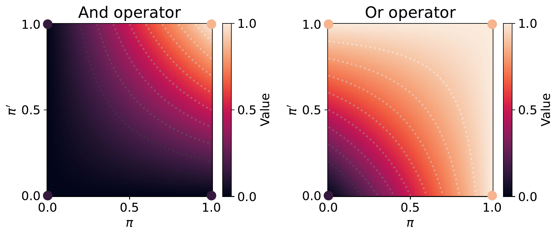
We can equivalently write the and, or and not operators as and(π,π′)or(π,π′)not(π)=π⋅π′=π+π′−π⋅π′=1−π. These are extensions of the previous definitions: we can use them as functions from [0,1]×[0,1]→[0,1], as illustrated in Fig. 5.3. This means that we can use the soft comparison operators defined in Section 5.2 to obtain π,π′∈[0,1]. Likewise, we can define continuous extensions of all and any, which are functions from [0,1]K to [0,1], as all(π)any(π)=i=1∏Kπi=1−i=1∏K(1−πi).
Figure 5.3: The Boolean and and or operators are functions from {0,1}×{0,1} to {0,1} (corners in the figure) but their continuous extensions and(π,π′):=π⋅π′ as well as or(π,π′):=π+π′−π⋅π′ define a function from [0,1]×[0,1] to [0,1].
From a probabilistic perspective, if we let Y and Y′ be two independent random variables distributed according to Bernoulli distributions with parameters π and π′, then and(π,π′)or(π,π′)not(π)=P(Y=1∩Y′=1)=P(Y=1)⋅P(Y′=1)=P(Y=1∪Y′=1)=P(Y=1)+P(Y′=1)−P(Y=1∩Y′=1)=P(Y=1)+P(Y′=1)−P(Y=1)P(Y′=1)=P(Y=1)=1−P(Y=1). In probability theory, these correspond to the product rule of two independent variables, the addition rule, and the complement rule.
Likewise, if we let Y=(Y1,…,YK)∈{0,1}K be a random variable distributed according to a multivariate Bernoulli distribution with parameters π=(π1,…,πK), then all(π)any(π)=P(Y1=1∩⋯∩YK=1)=i=1∏KP(Yi=1)=P(Y1=1∪⋯∪YK=1)=1−P(¬(Y1=1∪⋯∪YK=1))=1−P(Y1=1∩⋯∩YK=1)=1−i=1∏K(1−P(Yi=1)). These are the chain rule of probability and the addition rule of probability for K independent variables.
5.5.2 Triangular norms and co-norms
More generally, in the fuzzy logic literature (Jayaram and Baczynski, 2008; Klir and Yuan, 1995), the concepts of triangular norms and co-norms have been introduced to provide continuous relaxations of the and and or operators, respectively.
Definition 5.1(Triangular norms and conorms)
A triangular norm, a.k.a. t-norm, is a function from [0,1]×[0,1] to [0,1] which is commutative, associative, neutral w.r.t. 1 and is monotone, meaning that t(π,π′)≤t(τ,τ′) for all π≤τ and π′≤τ′. A triangular conorm, a.k.a. t-conorm, is defined similarly but is neutral w.r.t. 0.
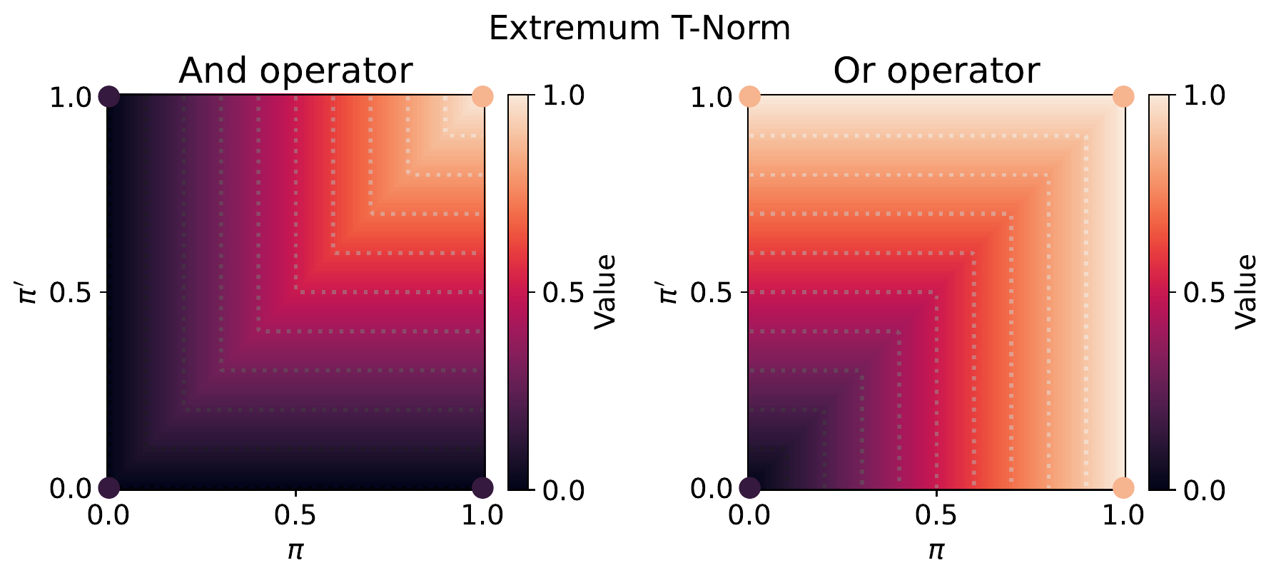
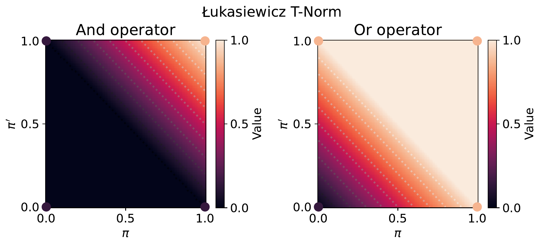
The previously-defined probabilistic extensions of and and or are examples of triangular norms and conorms. More examples are given in Table 5.1. Thanks to the associative property of these operators, we can generalize them to vectors π∈[0,1]K to define continuous extensions of the all and any operators, as shown in Table 5.2. For more examples and analysis, see for instance van Krieken (2024, 2 and 3).
Figure 5.4: Alternative relaxations of the Boolean and and or operators using triangular norms (t-norms).
Table 5.1: Examples of triangular norms and conorms, which are continuous relaxations of the and and or operators, respectively. More instances can be obtained by smoothing out the min and max operators.
t-norm (relaxed and)
t-conorm (relaxed or)
Probabilistic
π⋅π′
π+π′−π⋅π′
Extremum
min(π,π′)
max(π,π′)
Łukasiewicz
max(π+π′−1,0)
min(π+π′,1)
Table 5.2: Continuous extensions of the all and any operators.
All (∀)
Any (∃)
Probabilistic
∏i=1Kπi
1−∏i=1K(1−πi)
Extremum
min(π1,…,πK)
max(π1,…,πK)
Łukasiewicz
max(∑i=1Kπi−(K−1),0)
min(∑i=1Kπi,1)
5.6 If-else statements
An if-else statement executes different code depending on a condition. Formally, we can define the ifelse:{0,1}×V×V→V function by ifelse(π,v1,v0):={v1v0 if π=1 if π=0=π⋅v1+(1−π)⋅v0.(5.3) The π variable is called the predicate. It is a binary (Boolean) variable, making the function ifelse undefined if π∈{0,1}. The function is therefore discontinuous and nondifferentiable w.r.t. π∈{0,1}. On the other hand, v0∈V and v1∈V, which correspond to the false and true branches, can be continuous variables. If π=1, the function is linear w.r.t. v1 and constant w.r.t. v0. Conversely, if π=0, the function is linear w.r.t. v0 and constant w.r.t. v1. We now discuss how to differentiate through ifelse.
5.6.1 Differentiating through branch variables
For π∈{0,1} fixed, ifelse(π,v1,v0) is a valid function w.r.t. v1∈V and v0∈V, and can therefore be used as a node in a computational graph (Section 8.3). Due to the linearity w.r.t. v1 and v0, we obtain that the Jacobians w.r.t. v1 and v0 are ∂v0ifelse(π,v1,v0):={0I if π=1 if π=0=(1−π)⋅I and ∂v1ifelse(π,v1,v0):={I0 if π=1 if π=0=π⋅I, where I is the identity matrix of appropriate size. Most of the time, if-else statements are composed with other functions. Let g1:U1→V and g0:U0→V be differentiable functions. We then define v1:=g1(u1) and v0:=g0(u0), where u1∈U1 and u0∈U0. The composition of ifelse, g1 and g0 is then the function f:{0,1}×U1×U0→V defined by f(π,u1,u0):=ifelse(π,g1(u1),g0(u0))=π⋅g1(u1)+(1−π)⋅g0(u0). We obtain that the Jacobians are ∂u1f(π,u1,u0)=π⋅∂g1(u1) and ∂u0f(π,u1,u0)=(1−π)⋅∂g0(u0). As long as g1 and g0 are differentiable functions, we can therefore differentiate through the branch variables u1 and u0 without any issue. More problematic is the predicate variable π, as we now discuss.
5.6.2 Differentiating through predicate variables
The predicate variable π is binary and therefore cannot be differentiated directly. However, π can be the output of a comparison operator. For example, suppose we want to express the function fh:R×U1×U0→V defined by fh(p,u1,u0):={g1(u1)g0(u0) if p≥0 otherwise . Using our notation, this can be rewritten as fh(p,u1,u0):=ifelse(gt(p,0),g1(u1),g0(u0))=ifelse(step(p),g1(u1),g0(u0))=step(p)g1(u1)+(1−step(p))g0(u0). The Heaviside step function has a discontinuity at p=0, but it is continuous and differentiable with derivative step′(p)=0 for all p=0. The function fh therefore has null derivativew.r.t. p=0, ∂pfh(p,u1,u0)=∂1fh(p,u1,u0)=step′(p)(g1(u1)−g0(u0))=0. In other words, while fh has well-defined derivatives w.r.t. p for p=0, the derivatives are uninformative. As another example, let us now consider the function gh(u1,u0):=fh(t(u1),u1,u0), for some differentiable function t. This time, u1 influences both the predicate and the true branch. Then, using Proposition 2.8, we obtain ∂u1gh(u1,u0)=∂t(u1)∂1fh(t(u1),u1,u0)+∂2fh(t(u1),u1,u0)=∂2fh(t(u1),u1,u0). In other words, the derivatives of the predicate t(u1) do not influence the derivatives of gh.
5.6.3 Continuous relaxations
Fortunately, we recall that ifelse(π,v1,v0)=π⋅v1+(1−π)⋅v0. This function is perfectly well-defined, even if π∈[0,1], instead of π∈{0,1}. That is, this definition is an extension of Eq. (5.3) from the discrete set {0,1} to the continuous unit segment [0,1]. We saw that gt(a,b)≈gtσ(a,b):=sigmoidσ(a−b)∈[0,1], where we use sigmoidσ to denote a differentiable S-shaped function mapping R to [0,1]. For instance, we can use the logistic function or the standard Gaussian’s CDF. If we now define fs(p,u1,u0):=ifelse(gtσ(p,0),g1(u1),g0(u0))=ifelse(sigmoidσ(p),g1(u1),g0(u0))=sigmoidσ(p)g1(u1)+(1−sigmoidσ(p))g0(u0),(5.4) the Jacobian becomes ∂pfs(p,u1,u0)=sigmoidσ′(p)(g1(u1)−g0(u0)). If sigmoidσ=logistic(⋅/σ) or sigmoidσ=Φ(⋅/σ), the Jacobian is non-null everywhere, allowing gradients to backpropagate through the computational graph. This is an example of smoothing as studied in Part IV.
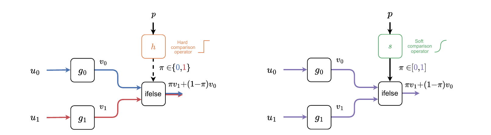
Figure 5.5: Computation graphs of programs using if-else statements with either hard or soft comparison operators. By using a hard comparison operator (step function, left panel) the predicate π is a discrete variable (represented by a dashed line). Depending on the value (0 or 1) of the predicate π, only one branch (red or blue) contributes to the output. Derivatives along a path of continuous variables (dense lines) can be computed. However, discrete variables such as the predicate prevent the propagation of meaningful derivatives. By using a soft comparison operator (sigmoid, right panel), the predicate is a continuous variable and derivatives with respect to the input p can be taken. In this case both branches (corresponding to g0 and g1) contribute to the output and therefore need to be evaluated.
Probabilistic perspective
From a probabilistic perspective, we can view Eq. (5.4) as the expectation of gi(ui), where i∈{0,1} is a binary random variable distributed according to a Bernoulli distribution with parameter π=sigmoidσ(p): fs(p,u1,u0)=Ei∼Bernoulli(sigmoidσ(p))[gi(ui)]. Taking the expectation over the two possibles branches makes the function differentiable with respect to p, since sigmoidσ(p) is differentiable. Of course, this comes at the cost of evaluating both branches, instead of a single one. The probabilistic perspective suggests that we can also compute the variance if needed as =Vi∼Bernoulli(sigmoidσ(p))[gi(ui)]Ei∼Bernoulli(sigmoidσ(p))[(fs(p,u1,u0)−gi(ui))2]. The probabilistic viewpoint also suggests different scales at which a smoothing can be defined as illustrated in Fig. 5.6.
Another perspective (Petersen et al., 2021) is based on the logistic distribution. Indeed, if P is a random variable following a logistic distribution with mean p and scale 1, we saw in Remark 3.1 that the CDF is P(P≤0)=logistic(−p)=1−logistic(p) and therefore fs(p,u1,u0)=ifelse(logistic(p),g1(u1),g0(u0))=logistic(p)g1(u1)+(1−logistic(p))g0(u0)=P(P>0)⋅g1(u1)+P(P≤0)⋅g0(u0).
Remark 5.1(Global versus local smoothing)
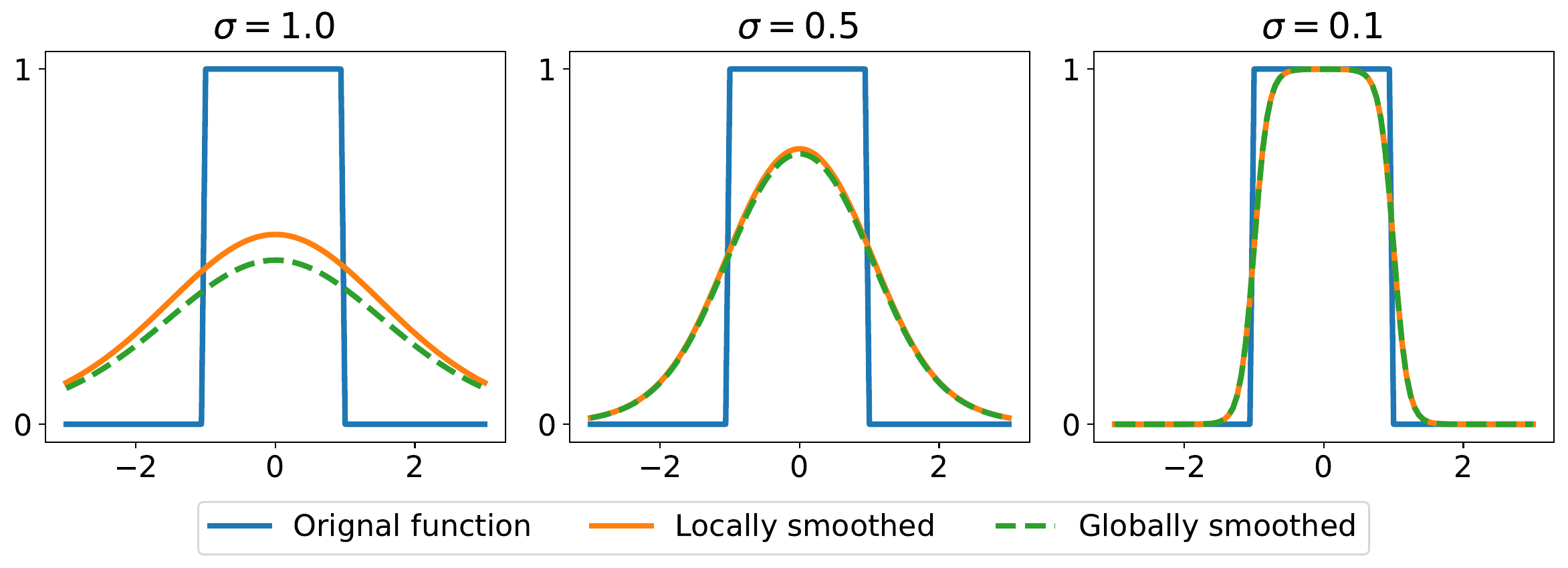
Consider the function f(x,y,z):={yzifa≤x≤botherwise. The derivatives w.r.t. y and z are well-defined. The derivative w.r.t. x on the other hand is not well-defined since it involves comparison operators and the logical operator and. Using our notation, we can rewrite the function as f(x,y,z)=ifelse(and(gt(x,a),lt(x,b)),y,z). A local smoothing approach consists in replacing gt and lt by gtσ and ltσ locally in the program: fσloc(x,y,z):=ifelse(and(gtσ(x,a),ltσ(x,b)),y,z)=πaπby+(1−πaπb)z where πaπb:=sigmoidσ(x−a):=sigmoidσ(b−x), for any sigmoid function sigmoidσ. A global smoothing approach instead uses the expectation of the entire program fσglob(x,y,z):=EZ[ifelse(and(gt(x+σZ,a),lt(x+σZ,b)),y,z)]=ifelse(π,y,z) where π:=EZ[and(gt(x+σZ,a),lt(x+σZ,b))]=P(a≤x+σZ≤b)=sigmoidσ(b−x)−sigmoidσ(a−x)=πb−πa, for sigmoidσ the CDF of σZ. We therefore obtain fσglob(x,y,z)=(πb−πa)y+(1−(πb−πa))z. The difference stems from the fact that the local approach smoothes out a≤x and x≤b independently (treating 1X≥a and 1X≤b as independent random variables), while the global approach smoothes out a≤x≤b simultaneously. In practice, both approaches approximate the original function well as σ→0 and coincide for σ sufficiently small as illustrated in Fig. 5.6.
Figure 5.6: Global versus local smoothing approaches on a gate function f(x):=1 if x∈[−1,1], and f(x):=0 otherwise. In our notation, we can write f(x)=ifelse(and(gt(x,−1),lt(x,1)),1,0). A local approach smoothes out gt and lt separately. A global approach uses the expectation of the whole program, see Remark 5.1. We observe that, though the approaches differ for large σ, they quickly coincide for smaller σ.
5.7 Else-if statements
In the previous section, we focused on if-else statements: conditionals with only two branches. We now generalize our study to conditionals including else-if statements, that have K branches.
5.7.1 Encoding K branches
For conditionals with only 2 branches, we encoded the branch that the conditional needs to take using the binary variable π∈{0,1}. For conditionals with K branches, we need a way to encode which of the K branches the conditional needs to take. To do so, we can use a vector π∈{e1,…,eK}, where ei denotes the standard basis vector (a.k.a. one-hot vector) ei:=(0,…,i1,…,0), a vector with a single one in the coordinate i and K−1 zeros. The vector ei is the encoding of a categorical variablei∈[K].
Combining booleans
To form such a vector π∈{e1,…,eK}, we can combine the previously-defined comparison and logical operators to define π=(π1,…,πK). However, we need to ensure that only one πi is non-zero. We give an example in Example 5.1.
Argmax and argmin operators
Another way to form π is to use the argmax and argmin operators argmax(p)argmin(p):=π∈{e1,…,eK}argmax⟨π,p⟩:=π∈{e1,…,eK}argmin⟨π,p⟩=argmax(−p). They can be seen as a natural generalization of the greater than and less than operators. In case of ties, we break them arbitrarily.
5.7.2 Conditionals
We can now express a conditional statement as the function cond:{e1,…,eK}×VK→V defined by cond(π,v1,…,vK):=⎩⎨⎧v1⋮vK if π=e1 if π=eK=i=1∑Kπivi.(5.5) Similarly to the ifelse function, the cond function is discontinuous and nondifferentiable w.r.t. π∈{e1,…,eK}. However, given π=ei fixed for some i, the function is linear in vi and constant in vj for j=i. We illustrate how to express a simple example, using this formalism.
Example 5.1(Soft-thresholding operator)
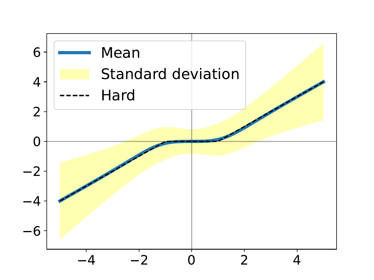
The soft-thresholding operator (see also Section 16.4) is a commonly-used operator to promote sparsity. It is defined by SoftThreshold(u,λ):=⎩⎨⎧0u−λu+λ if ∣u∣≤λ if u≥λ if u≤−λ. To express it in our formalism, we can define π∈{e1,e2,e3} using comparison operators as π:=(lt(∣u∣,λ),gt(u,λ),lt(u,−λ))=(step(λ−∣u∣),step(u−λ),step(−u−λ)). Equivalently, we can also define π using an argmax operator as π:=argmax((λ−∣u∣,u−λ,−u−λ)). In case of ties, which happens at ∣u∣=λ, we keep only one non-zero coordinate in π. We can then rewrite the operator as SoftThreshold(u,λ)=cond(π,0,u−λ,u+λ). As we will see, replacing argmax with softargmax induces a categorical distribution over the three possible branches. The mean value can be seen as a smoothed out version of the operator, and we can also compute the standard deviation, as illustrated in Fig. 5.7.
Figure 5.7: A conditional with three branches: the soft-thresholding operator (see Example 5.1). It is a piecewise linear function (dotted black line). Using a softargmax, we can induce a categorical probability distribution over the three branches. The expected value (blue line) can be seen as a smoothed out version of the operator. The induced distribution allows us to also compute the standard deviation.
5.7.3 Differentiating through branch variables
For π fixed, cond(π,v1,…,vK) is a valid function w.r.t. vi, and can therefore again be used as a node in a computational graph. Due to the linearity w.r.t. vi, we obtain that the Jacobian w.r.t. vi is ∂vicond(π,v1,…,vK):={I0 if π=ei if π=ei. Let gi:Ui→V be a differentiable function and ui∈Ui. If we define the composition f(π,u1,…,uK):=cond(π,g1(u1),…,gK(uK)), we then obtain that the Jacobian w.r.t. ui is ∂uif(π,u1,…,uK):={∂gi(ui)0 if π=ei if π=ei. As long as the gi functions are differentiable, we can therefore differentiate through the branch variables ui for π fixed.
5.7.4 Differentiating through predicate variables
As we saw, π can be obtained by combining comparison and logical operators, or it can be obtained by argmax and argmin operators. We illustrate here why these operators are problematic. For example, suppose we want to express the function fa(p,u1,…,uK):=⎩⎨⎧v1⋮vK if p=e1 if p=eK. In our notation, this can be expressed as fa(p,u1,…,uK):=cond(argmax(p),g1(u1),…,gK(uK)), As for the ifelse case, the Jacobian w.r.t. p is null almost everywhere, ∂pfa(p,u1,…,uK)=0.
5.7.5 Continuous relaxations
Similarly to the Heaviside step function, the argmax and argmin functions are piecewise constant, with discontinuities in case of ties. Their Jacobians are zero almost everywhere, and undefined in case of ties. Therefore, while their Jacobian is well-defined almost everywhere, they are uninformative and prevent gradient backpropagation. We can replace the argmax with a softargmaxsoftargmax(p):=∑i=1Kexp(pi)exp(p)∈△K and similarly softargmin(p):=softargmax(−p)∈△K. Other relaxations of the argmax are possible, as discussed in Section 13.7. See also Section 14.5.3 for the perturbation perspective.
Fortunately, the definition cond(π,v1,…,vK)=i=1∑Kπivi is perfectly valid if we use π∈△K instead of π∈{e1,…,eK}, and can therefore be seen as an extension of Eq. (5.5). If we now define fs(p,u1,…,uK):=cond(softargmax(p),g1(u1),…,gK(uK))=i=1∑K[softargmax(p)]i⋅gi(ui),(5.6) the Jacobian becomes ∂pfs(p,u1,…,uK)=∂softargmax(p)(g1(u1),…,gK(uK)), which is non-null everywhere, allowing gradients to backpropagate through the computational graph.
Probabilistic perspective
From a probabilistic perspective, we can view Eq. (5.6) as the expectation of gi(ui), where i∈[K] is a categorical random variable distributed according to a categorical distribution with parameter π=softargmax(p): fs(p,u1,…,uK)=Ei∼Categorical(softargmax(p))[gi(ui)]. Taking the expectation over the K possible branches makes the function differentiable with respect to p, at the cost of evaluating all branches, instead of a single one. Similarly as for the if-else case, we can compute the variance if needed as =Vi∼Categorical(softargmax(p))[gi(ui)]Ei∼Categorical(softargmax(p))[(fs(p,u1,…,uK)−gi(ui))2]. This is illustrated in Fig. 5.7.
5.8 For loops
For loops are a control flow for sequentially calling a fixed number K of functions, reusing the output from the previous iteration. In full generality, a for loop can be written as follows.
Algorithm 5.1:r=forloop(s0)
fork:=1,…,Kdo
sk:=fk(sk−1)
r:=sK
As illustrated in Fig. 5.8, this defines a computation chain. Assuming the functions fk are all differentiable, this defines a valid computation graph, we can therefore use automatic differentiation to differentiate forloopw.r.t. its input s0. Feedforward networks, reviewed in Section 4.2, can be seen as parameterized for loops, i.e., fk(sk−1):=gk(sk−1,wk), for some differentiable function gk.
Example 5.2(Unrolled gradient descent)
Suppose we want to minimize w.r.t. w the function L(w,λ):=N1i=1∑Nℓ(h(xi,w),yi)+2λ∥w∥22. Given an initialization w0, gradient descent (Section 16.1) performs iterations of the form wk=f(wk−1,γk,λ):=wk−1−γk∇1L(wk−1,λ). Gradient descent can therefore be expressed as a for loop with fk(wk−1):=f(wk−1,γk,λ). This means that we can differentiate through the iterations of gradient descent, as long as f is differentiable, meaning that L is twice differentiable. This is useful for instance to perform gradient-based optimization of the hyperparameters γk or λ. This is a special case of bilevel optimization; see also Chapter 11.
Example 5.3(Bubble sort)
Bubble sort is a simple sorting algorithm that works by repeatedly swapping elements if necessary. Mathematically, swapping two elements i and j can be written as a function from RN×[N]×[N] to RN defined by swap(v,i,j):=v+(vj−vi)ei+(vi−vj)ej. We can then write bubble sort as fori:=1,…,Ndoforj:=1,…,N−i−1dov′:=swap(v,j,j+1)π:=step(vj−vj+1)v←ifelse(π,v′,v) Replacing the Heaviside step function with the logistic function gives a smoothed version of the algorithm.
Figure 5.8: A for loop forms a computation chain. A feed forward network can be seen as a parameterized for loop, where each function fk depends on some parameters wk.
Figure 5.9: Computation graph of the scan function. Sequence-to-sequence RNNs can be seen as a parameterized scan function.
5.9 Scan functions
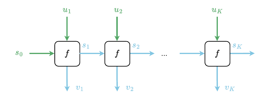
Scan is a higher-order function (meaning a function of a function) originating from functional programming. It is useful to perform an operation f on individual elements uk while carrying the result sk of that operation to the next iteration.
Algorithm 5.2:r=scan(s0,u1,…,uK)
fork:=1,…,Kdo
sk,vk:=f(sk−1,uk)
r:=(sK,v1,…,vK)
As illustrated in Fig. 5.9, this again defines a valid computational graph and can be differentiated through using autodiff, assuming the function f is differentiable. Sequence-to-sequence RNNs, reviewed in Section 4.7, can be seen as a parameterized scan. An advantage of this abstraction is that parallel scan algorithms have been studied extensively in computer science (Blelloch, 1989; Sengupta et al., 2010).
Example 5.4(Prefix sum)
Scan can be seen as a generalization of the prefix sum (a.k.a. cumulative sum) from the addition to any binary operation. Indeed, a prefix sum amounts to perform v1v2v3:=u1:=u1+u2:=u1+u2+u3⋮ which can be expressed as a scan by defining vkf(sk−1,uk):=sk−1+uk:=(vk,vk) starting from s0=0 (sK and vK are redundant in this case).
5.10 While loops
5.10.1 While loops as cyclic graphs
A while loop is a control flow used to repeatedly perform an operation, reusing the output of the previous iteration, until a certain condition is met. Suppose f:S→{0,1} is a function to determine whether to stop (π=1) or continue (π=0) and g:S→S is a function for performing an operation. Then, without loss of generality, a while loop can be written as follows.
Algorithm 5.3:r=whileloop(s)
π←f(s)
whileπ=0do
s←g(s)
π←f(s)
r:=s
This definition is somewhat cyclic, as we used the while keyword. However, we can equivalently rewrite the algorithm recursively.
Algorithm 5.4:r=whileloop(s)
π:=f(s)
ifπ=0then
r:=s
else
r:=whileloop(g(s))
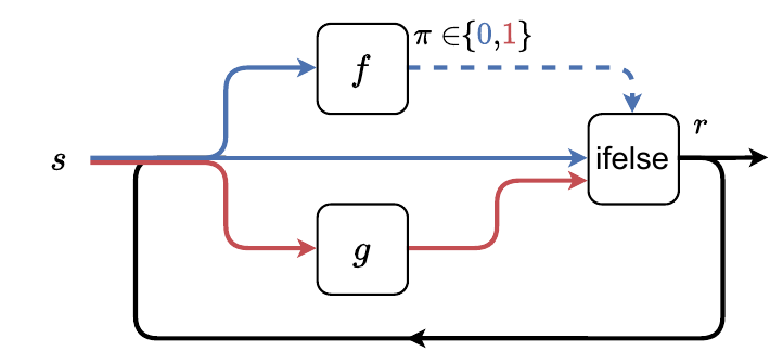
Unlike for loops and scan, the number of iterations of while loops is not known ahead of time, and may even be infinite. In this respect, a while loop can be seen as a cyclic graph, as illustrated in Fig. 5.10.
Figure 5.10: A while loop can be represented as a cyclic graph. The while loop stops if π=1 and performs another iteration s←g(s), π←f(s) if π=0.
Importance of lazy evaluation
We can also implement Algorithm 5.4 in terms of the ifelse function defined in Section 5.6 as r:=ifelse(f(s),whileloop(g(s)),s)=f(s)⋅whileloop(g(s))+(1−f(s))⋅s. However, to avoid an infinite recursion, it is crucial that ifelse supports lazy evaluation. That is, whileloop(g(s)) in the definition above should be evaluated if and only if π=f(s)=1. In other words, the fact that f(s)∈{0,1} is crucial to ensure that the recursion is well-defined.
5.10.2 Unrolled while loops
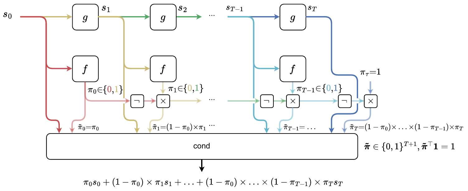
To avoid the issues with unbounded while loops, we can enforce that a while loop stops after T iterations, i.e., we can truncate the while loop. Unrolling Algorithm 5.4 gives (here with T=3) π0:=f(s0)ifπ0=1thenr:=s0elses1:=g(s0),π1:=f(s1)ifπ1=1thenr:=s1elses2:=g(s1),π2:=f(s2)ifπ2=1thenr:=s2elser:=s3:=g(s2) Using the ifelse function, we can rewrite it as r=ifelse(π0,s0,ifelse(π1,s1,ifelse(π2,s2,s3))) which is itself equivalent to r=π0s0+(1−π0)[π1s1+(1−π1)[π2s2+(1−π2)s3]]=π0s0+(1−π0)π1s1+(1−π0)(1−π1)π2s2+(1−π0)(1−π1)(1−π2)s3. More generally, for T∈N, the formula is r=i=0∑T((1−π0)…(1−πi−1))πisi=i=0∑T(j=0∏i−1(1−πj))πisi, where we defined siπi:=g(si−1):=gi(s0):=i timesg∘⋯∘g(s0)∈S:=f(si)∈{0,1}. See also (Petersen et al., 2021). If we further define the shorthand notation π~0π~i:=π0:=(j=0∏i−1(1−πj))πii∈{1,…,T}, so that π~:=(π~0,π~1,…,π~T)∈△T+1 is a discrete probability distribution containing the probabilities to stop at each of the T iterations, we can rewrite the output of a truncated while using a conditional, r=cond(π~,s0,s1,…,sT)=t=0∑Tπ~tst. This is illustrated in Fig. 5.11.
Figure 5.11: Computation graph of an unrolled truncated while loop. As in Fig. 5.5, we depict continuous variables in dense lines and discrete variables in dashed lines. The output of a while loop with at most T iterations can be written as a conditional with T+1 branches, cond(π~,s0,…,sT)=∑t=0Tπ~tst.
Example 5.5(Computing the square root using Newton’s method)
Computing the square root x of a real number x>0 can be cast as a root finding problem, which we can solve using Newton’s method. Starting from an initialization s0, the iterations read si+1:=g(si):=21(si+six). To measure the error on iteration i, we can define ε(si):=21(si2−x)2. As a stopping criterion, we can then use πi:={10 if ε(si)≤τ otherwise =step(τ−ε(si)), where 0<τ≪1 is an error tolerance and step is the Heaviside step function.
5.10.3 Markov chain perspective
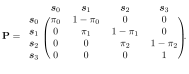
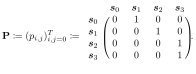
Given the function g:S→S and the initialization s0∈S, a while loop can only go through a discrete set of values s0,s1,s2,… defined by si=g(si−1). This set is potentially countably infinite if the while loop is unbounded, and finite if the while loop is guaranteed to stop. Whether the loop moves from the state si to the state si+1, or stays at si, is determined by the stopping criterion πi∈{0,1}. To model the state of the while loop, we can then consider a Markov chain with a discrete space {s0,s1,s2,…}, which we can always identify with {0,1,2,…}, with transition probabilities P(St+1=si∣St=sj)=pi,j:=⎩⎨⎧πi(1−πi)0 if i=j if i=j+1 otherwise , and initial state S0=s0. Here, St is the value at iteration t of the loop. Note that since πi∈{0,1}, the pi,j values are “degenerate” probabilities. However, this framework lets us generalize to a smooth version of the while loop naturally. To illustrate the framework, if the while loop stops at T=3, the transition probabilities can be cast as a matrix The output r of the while-loop is determined by the time at which the state stays at the same value I=min{i∈{1,2,…}s.t.Si=Si−1}. Note that I itself is a random variable, as it is defined by the Si variables. It is called a stopping time. The output of the chain is then r=E[SI]=i=1∑+∞P(I=i)E[Si∣I=i]=i=1∑+∞P(I=i)si−1=i=1∑+∞j=0∏i−2(1−πj)πi−1si−1=i=0∑+∞j=0∏i−1(1−πj)πisi. Because the stopping time is not known ahead of time, the sum over i goes from 0 to ∞. However, if we enforce in the stopping criterion that the while loop runs no longer than T iterations, by setting πi:=or(f(si),eq(i,T))∈{0,1}, we then naturally recover the expression found by unrolling the while loop before, r=E[SI]=i=0∑Tj=0∏i−1(1−πj)πisi. For example, with T=3, the transition probability matrix is
Smoothed while loops
With the help of this framework, we can backpropagate even through the while loop’s stopping criterion, provided that we smooth out the predicate. For example, we saw that the stopping criterion in Example 5.5 is f(si)=step(τ−ε(si)) and therefore πi:=or(f(si),eq(i,T))∈{0,1}. Due to the step function, the derivative of the while loop with respect to τ will always be 0, just like it was the case for if-else statements. If we change the stopping criterion to f(si)=sigmoid(τ−ε(si)), we then have (recall that or is well defined on [0,1]×[0,1]) πi:=or(f(si),eq(i,T))∈[0,1]. With sigmoid, we obtain more informative derivatives. In particular, with sigmoid=logistic, the derivatives w.r.t. τ are always non-zero. The smoothed output is expressed as before as the expectation r=E[SI]=i=0∑Tj=0∏i−1(1−πj)πisi where πi:=sigmoid(τ−ε(si)). Instead of enforcing a number T of iterations, it is also possible to stop when the probability of stopping becomes high enough (Petersen et al., 2021), assuming that the probability of stopping converges to 1.
5.11 Summary
For conditionals, we saw that differentiating through the branch variables is not problematic given a fixed predicate.
However, for the predicate variable, we saw that a differentiable relaxation is required to avoid null derivatives.
We introduced soft comparison operators in a principled manner, using a stochastic process perspective, as well as the continuous extension of logical operators.
For loops and scan define valid computational graphs, as their number of iterations is fixed ahead of time. Feedforward networks and RNNs can be seen as parameterized for loops and scan, respectively.
Unlike for loops and scan, the number of iterations of while loops is not known ahead of time and may even be infinite. However, unrolled while loops define valid directed acyclic graphs. We defined a principled way to differentiate through the stopping criterion of a while loop, thanks to a Markov chain perspective.

 The output of the while-loop is determined by the time at which the state stays at the same value Note that itself is a random variable, as it is defined by the variables. It is called a stopping time. The output of the chain is then Because the stopping time is not known ahead of time, the sum over goes from to . However, if we enforce in the stopping criterion that the while loop runs no longer than iterations, by setting we then naturally recover the expression found by unrolling the while loop before, For example, with , the transition probability matrix is